Lecture 10
In this lecture, we will discuss increasingly popular packages and methods in R that are intended to make code more readable or make otherwise complicated tasks simpler. No package listed here is included in the base R installation, and must be installed from CRAN. That said, they can make working in R much easier.
magrittr and the Pipe Operator
Let’s say that you have a long list of tasks that you want to perform on a data set. For example, you may want to take a data set, subset it, fit a linear model to it, and then get the coefficients. There are a few ways to do these four steps:
- Perform them all in one line, like so (for the
irisdata set):
coefficients(lm(Sepal.Length ~ Sepal.Width,
                data = subset(iris, select = -c(Species),
                              subset = Species == "virginica")))
## (Intercept) Sepal.Width
## 3.9068365 0.9015345- Perform each step on its own line, saving the results of the previous step and using the object you created in the next step:
iris_subset <- subset(iris, select = -c(Species),
                      subset = Species == "virginica")
mod <- lm(Sepal.Length ~ Sepal.Width, data = iris_subset)
coefficients(mod)
## (Intercept) Sepal.Width
## 3.9068365 0.9015345Not everyone is satisfied with this approach. The first can become quite long, and furthermore, you need to effectively read from right to left in order to understand what was done. The second approach requires keeping track of what each object in each step is, and thus can also be confusing.
The magrittr package, though, provides a third option: the pipe operator, %>%. The logic of the operator is simple: x %>% f == f(x). In other words, x becomes the first argument passed to the function f(). If f() takes multiple arguments, then the following holds: x %>% f(y) == f(x, y). If you wish for the pipe operator to pass the object on the left-hand side to something other than the first argument of f(), you can substitute . for the argument you wish to pass the object to: in other words, y %>% f(x, .) == f(x, y). You can also use . to pass the object on the left-hand side to a named argument, so y %>% f(x, foo = .) == f(x, foo = y).
While there’s no clear advantage to using the %>% operator when you’re dealing with just one object, when you wish to chain operations, it suddenly becomes very clear why many like using it. Here’s the above example repeated using %>%:
library(magrittr)
iris %>%
  subset(select = -c(Species), subset = Species == "versicolor") %>%
  lm(Sepal.Length ~ Sepal.Width, data = .) %>%
  coefficients
## (Intercept) Sepal.Width
## 3.5397347 0.8650777Furthermore, you can read the operation from left to right to understand what was done, and easily insert additional steps in the chain. Maybe you with to standardize the variables, wich is subtracting each observation by the mean and dividing by the standard deviation. It’s easy to insert that step into the above pipeline:
iris %>%
  subset(select = -c(Species), subset = Species == "versicolor") %>%
  scale %>%
  as.data.frame %>% # scale returns a matrix, but we want a data frame
  lm(Sepal.Length ~ Sepal.Width, data = .) %>%
  coefficients
## (Intercept) Sepal.Width
## 8.949085e-17 5.259107e-01If we were to “unwrap” the above code, it would be equivalent to:
# Have fun reading this and understanding what it does
coefficients(lm(Sepal.Length ~ Sepal.Width, data = as.data.frame(
scale(subset(iris, select = -c(Species),
subset = Species == "versicolor")))))## (Intercept) Sepal.Width
## 8.949085e-17 5.259107e-01magrittr includes operators other than the %>% operator, such as:
- The
%<>%operator, where the results of the function on the right are saved to the object on the left, orx %<>% f == {x <- x %>% f} == {x <- f(x)}:
# For demonstration purposes, make three copies of rivers
rivers1 <- rivers
rivers2 <- rivers
rivers3 <- rivers
# We will save the mean of rivers in these variables in three different ways
# 1: Without any pipe operators (By the way, did you know that if you wrap a
# command in parentheses, the object that is saved will also be printed in
# the console? This is a convenient way to both save and see the result of
# an operation.)
(rivers1 <- mean(rivers1))## [1] 591.1844# 2: With %>%
(rivers2 <- rivers2 %>% mean)## [1] 591.1844# 3: With %<>%
(rivers3 %<>% mean)## [1] 591.1844c(rivers1, rivers2, rivers3) %>% print## [1] 591.1844 591.1844 591.1844- The
%T>%operator, where the value on the left is returned instead of the operation on the right (useful if you want to see something about an intermediate step):
# Save current par settings
old_par <- par()
par(mfrow = c(1,2))
iris %>%
subset(select = -c(Species), subset = Species == "versicolor") %T>%
# The next step in the chain will not be passed to the following step, since
# above is %T>% rather than %>%; this is good because we don't want to use a
# plot object, just see it
plot(Sepal.Length ~ Sepal.Width, data = ., main = "Unscaled") %>%
scale %>%
as.data.frame %T>% # scale returns a matrix, but we want a data frame
# The next step in the chain will not be passed to the following step, since
# above is %T>% rather than %>%; this is good because we don't want to use a
# plot object, just see it
plot(Sepal.Length ~ Sepal.Width, data = ., main = "Scaled") %>%
lm(Sepal.Length ~ Sepal.Width, data = .) %>%
coefficients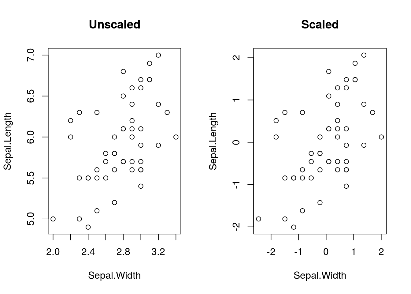
##  (Intercept)  Sepal.Width
## 8.949085e-17 5.259107e-01# Return to original settings
par(old_par)## Warning in par(old_par): graphical parameter "cin" cannot be set## Warning in par(old_par): graphical parameter "cra" cannot be set## Warning in par(old_par): graphical parameter "csi" cannot be set## Warning in par(old_par): graphical parameter "cxy" cannot be set## Warning in par(old_par): graphical parameter "din" cannot be set## Warning in par(old_par): graphical parameter "page" cannot be set- The
%$%operator works like%>%but also exposes the names of the object on the left-hand side to the operation on the right-hand side; in effect, it’s a combination of%>%andwith(). It other words, ifzis a variable inx(perhapsxis a data frame or list), thenx %$% f(z) == with(x, z %>% f) == with(x, f(z)):
# Intelligent use of the %$% operator allows us to avoid using the data argument of lm, making the pipeline even simpler
par(mfrow = c(1,2))

iris %>%
  subset(select = -c(Species), subset = Species == "versicolor") %>%
  scale %>%
  as.data.frame %$% # Now we don't need data = . ; there is an implicit with()
  lm(Sepal.Length ~ Sepal.Width) %>%
  coefficients
## (Intercept) Sepal.Width
## 8.949085e-17 5.259107e-01# Here is an equivalent, ugly one-line command
coefficients(with(
as.data.frame(
scale(
subset(iris, select = -c(Species), subset = Species == "versicolor"))),
lm(Sepal.Length ~ Sepal.Width)))## (Intercept) Sepal.Width
## 8.949085e-17 5.259107e-01You can learn more about magrittr and the pipe operator here.
dplyr: Subsetting With Power
Throughout this course, we have seen many methods for subsetting a data frame, including bracket notation (that is, df[x,y]) and, in particular, the subset() function. The bracket notation can easily become unruly (especially if you are using which()). subset() is much better, but the notation is not necessarily convenient and the function itself is slow and limited in use (it is basically a convenience method for the bracket notation). Furthermore, these functions will not do everything you want (say, order the rows of a data frame, or conveniently rename columns).
Hadley Wickham, the main creator of ggplot2, created a package called dplyr that provides alternative subsetting methods. The package is designed to support use of the %>% operator (magrittr is loaded in automatically when you load dplyr) with data manipulation functions. Also, while subset() is intended to work just with data frames and doesn’t provide any speed advantages, dplyr functions are not only often faster, they can work with objects other than data frames, such as a connection to a SQL data base (the logic of dplyr functions is similar in many ways to SQL logic, and with both can be modeled abstractly with relational algebra).
Basic subsetting using select() and filter()
The dplyr functions select() and filter() together give you all the capabilities of subset() in base R.
select(df, ...) chooses the columns from the data frame df to include in the output. You can make this selection exactly like you would using the select argument in subset() (with negative indices, :, or just listing out the columns you want).
filter(df, logical_statement) chooses the rows from the data frame df to include in the output, using syntax identical to that of the subset argument of the subset function. You write out a logical statement describing which rows you want, depending on column values.
Here are two ways to get the same data frame, using subset() and the dplyr functions.
# The subset way
subset(iris, select = Petal.Length:Species, subset = Species == "virginica" &
    Petal.Length > mean(Petal.Length))
## Petal.Length Petal.Width Species
## 101 6.0 2.5 virginica
## 102 5.1 1.9 virginica
## 103 5.9 2.1 virginica
## 104 5.6 1.8 virginica
## 105 5.8 2.2 virginica
## 106 6.6 2.1 virginica
## 107 4.5 1.7 virginica
## 108 6.3 1.8 virginica
## 109 5.8 1.8 virginica
## 110 6.1 2.5 virginica
## 111 5.1 2.0 virginica
## 112 5.3 1.9 virginica
## 113 5.5 2.1 virginica
## 114 5.0 2.0 virginica
## 115 5.1 2.4 virginica
## 116 5.3 2.3 virginica
## 117 5.5 1.8 virginica
## 118 6.7 2.2 virginica
## 119 6.9 2.3 virginica
## 120 5.0 1.5 virginica
## 121 5.7 2.3 virginica
## 122 4.9 2.0 virginica
## 123 6.7 2.0 virginica
## 124 4.9 1.8 virginica
## 125 5.7 2.1 virginica
## 126 6.0 1.8 virginica
## 127 4.8 1.8 virginica
## 128 4.9 1.8 virginica
## 129 5.6 2.1 virginica
## 130 5.8 1.6 virginica
## 131 6.1 1.9 virginica
## 132 6.4 2.0 virginica
## 133 5.6 2.2 virginica
## 134 5.1 1.5 virginica
## 135 5.6 1.4 virginica
## 136 6.1 2.3 virginica
## 137 5.6 2.4 virginica
## 138 5.5 1.8 virginica
## 139 4.8 1.8 virginica
## 140 5.4 2.1 virginica
## 141 5.6 2.4 virginica
## 142 5.1 2.3 virginica
## 143 5.1 1.9 virginica
## 144 5.9 2.3 virginica
## 145 5.7 2.5 virginica
## 146 5.2 2.3 virginica
## 147 5.0 1.9 virginica
## 148 5.2 2.0 virginica
## 149 5.4 2.3 virginica
## 150 5.1 1.8 virginica# The dplyr way
library(dplyr)##
## Attaching package: 'dplyr'## The following objects are masked from 'package:stats':
##
## filter, lag## The following objects are masked from 'package:base':
##
## intersect, setdiff, setequal, unioniris %>% filter(Species == "virginica" & Petal.Length > mean(Petal.Length)) %>%
select(Petal.Length:Species)## Petal.Length Petal.Width Species
## 1 6.0 2.5 virginica
## 2 5.1 1.9 virginica
## 3 5.9 2.1 virginica
## 4 5.6 1.8 virginica
## 5 5.8 2.2 virginica
## 6 6.6 2.1 virginica
## 7 4.5 1.7 virginica
## 8 6.3 1.8 virginica
## 9 5.8 1.8 virginica
## 10 6.1 2.5 virginica
## 11 5.1 2.0 virginica
## 12 5.3 1.9 virginica
## 13 5.5 2.1 virginica
## 14 5.0 2.0 virginica
## 15 5.1 2.4 virginica
## 16 5.3 2.3 virginica
## 17 5.5 1.8 virginica
## 18 6.7 2.2 virginica
## 19 6.9 2.3 virginica
## 20 5.0 1.5 virginica
## 21 5.7 2.3 virginica
## 22 4.9 2.0 virginica
## 23 6.7 2.0 virginica
## 24 4.9 1.8 virginica
## 25 5.7 2.1 virginica
## 26 6.0 1.8 virginica
## 27 4.8 1.8 virginica
## 28 4.9 1.8 virginica
## 29 5.6 2.1 virginica
## 30 5.8 1.6 virginica
## 31 6.1 1.9 virginica
## 32 6.4 2.0 virginica
## 33 5.6 2.2 virginica
## 34 5.1 1.5 virginica
## 35 5.6 1.4 virginica
## 36 6.1 2.3 virginica
## 37 5.6 2.4 virginica
## 38 5.5 1.8 virginica
## 39 4.8 1.8 virginica
## 40 5.4 2.1 virginica
## 41 5.6 2.4 virginica
## 42 5.1 2.3 virginica
## 43 5.1 1.9 virginica
## 44 5.9 2.3 virginica
## 45 5.7 2.5 virginica
## 46 5.2 2.3 virginica
## 47 5.0 1.9 virginica
## 48 5.2 2.0 virginica
## 49 5.4 2.3 virginica
## 50 5.1 1.8 virginica# The slice() function in dplyr allows selecting rows by index
iris %>% filter(Species == "virginica" & Petal.Length > mean(Petal.Length)) %>%
select(Petal.Length:Species) %>% slice(1:10)## # A tibble: 10 x 3
## Petal.Length Petal.Width Species
## <dbl> <dbl> <fct>
## 1 6 2.5 virginica
## 2 5.1 1.9 virginica
## 3 5.9 2.1 virginica
## 4 5.6 1.8 virginica
## 5 5.8 2.2 virginica
## 6 6.6 2.1 virginica
## 7 4.5 1.7 virginica
## 8 6.3 1.8 virginica
## 9 5.8 1.8 virginica
## 10 6.1 2.5 virginicaUnlike subset(), though, you can easily rename columns if necessary when using select(), like so:
iris %>% filter(Species == "virginica" & Petal.Length > mean(Petal.Length)) %>%
    select(Length = Petal.Length, Width = Petal.Width, Species) %>% slice(1:10)
## # A tibble: 10 x 3
## Length Width Species
## <dbl> <dbl> <fct>
## 1 6 2.5 virginica
## 2 5.1 1.9 virginica
## 3 5.9 2.1 virginica
## 4 5.6 1.8 virginica
## 5 5.8 2.2 virginica
## 6 6.6 2.1 virginica
## 7 4.5 1.7 virginica
## 8 6.3 1.8 virginica
## 9 5.8 1.8 virginica
## 10 6.1 2.5 virginicaIf you wish to rename the columns of an existing data frame without removing those not mentioned, use rename() instead:
(new_iris <- iris %>% select(Petal.Length:Species) %>% slice(1:10))## # A tibble: 10 x 3
## Petal.Length Petal.Width Species
## <dbl> <dbl> <fct>
## 1 1.4 0.2 setosa
## 2 1.4 0.2 setosa
## 3 1.3 0.2 setosa
## 4 1.5 0.2 setosa
## 5 1.4 0.2 setosa
## 6 1.7 0.4 setosa
## 7 1.4 0.3 setosa
## 8 1.5 0.2 setosa
## 9 1.4 0.2 setosa
## 10 1.5 0.1 setosanew_iris %>% rename(Length = Petal.Length, Width = Petal.Width)## # A tibble: 10 x 3
## Length Width Species
## <dbl> <dbl> <fct>
## 1 1.4 0.2 setosa
## 2 1.4 0.2 setosa
## 3 1.3 0.2 setosa
## 4 1.5 0.2 setosa
## 5 1.4 0.2 setosa
## 6 1.7 0.4 setosa
## 7 1.4 0.3 setosa
## 8 1.5 0.2 setosa
## 9 1.4 0.2 setosa
## 10 1.5 0.1 setosaAdding new variables with mutate()
Suppose you have a data frame and you want to add a new variable; perhaps you want to track the difference between Sepal.Length and Sepal.Width in the iris data set. mutate() (which is similar to the transform() function in base R) will allow for easily adding new variables in a data frame using existing variables. Suppose the data frame df contains the variables x and y. The call mutate(df, z = f(x,y)) will return a data frame identical to df but including a new variable z which is the result of applying f to the entry of the variable x and y to each row (note that f could be an expressions; say, subtraction). (Bear in mind that this works row-wise). If you want to return a data frame that only includes z (it does not include the original columns), use the transmute() function instead (not demonstrated).
iris %>% select(Petal.Length:Species) %>% filter(Species == "versicolor") %>%
    mutate(Difference = Petal.Length - Petal.Width, Ratio = Petal.Length/Petal.Width) %>%
    head
## Petal.Length Petal.Width Species Difference Ratio
## 1 4.7 1.4 versicolor 3.3 3.357143
## 2 4.5 1.5 versicolor 3.0 3.000000
## 3 4.9 1.5 versicolor 3.4 3.266667
## 4 4.0 1.3 versicolor 2.7 3.076923
## 5 4.6 1.5 versicolor 3.1 3.066667
## 6 4.5 1.3 versicolor 3.2 3.461538Other useful dplyr functions
I will mention three other functions you may find handy. The summarize() function will create a data frame with one row that contains requested numerical summaries, with the user specifying how to compute those summaries in the function call. An example is shown below:
iris %>% summarize(sepal_mean = mean(Sepal.Length), sepal_sd = sd(Sepal.Length),
    sepal_Q1 = quantile(Sepal.Width, 0.25), versicolor_count = sum(Species ==
        "versicolor"))
## sepal_mean sepal_sd sepal_Q1 versicolor_count
## 1 5.843333 0.8280661 2.8 50Finally, the functions sample_n() and sample_frac() allow for choosing random rows from a data frame, with sample_n() allowing you to set the number of rows you desire, and sample_frac() the fraction of rows from the original data frame you want. They are demonstrated below:
iris %>% sample_n(10)## Sepal.Length Sepal.Width Petal.Length Petal.Width Species
## 44 5.0 3.5 1.6 0.6 setosa
## 49 5.3 3.7 1.5 0.2 setosa
## 41 5.0 3.5 1.3 0.3 setosa
## 134 6.3 2.8 5.1 1.5 virginica
## 70 5.6 2.5 3.9 1.1 versicolor
## 71 5.9 3.2 4.8 1.8 versicolor
## 121 6.9 3.2 5.7 2.3 virginica
## 97 5.7 2.9 4.2 1.3 versicolor
## 96 5.7 3.0 4.2 1.2 versicolor
## 93 5.8 2.6 4.0 1.2 versicoloriris %>% sample_frac(.15)## Sepal.Length Sepal.Width Petal.Length Petal.Width Species
## 137 6.3 3.4 5.6 2.4 virginica
## 105 6.5 3.0 5.8 2.2 virginica
## 110 7.2 3.6 6.1 2.5 virginica
## 26 5.0 3.0 1.6 0.2 setosa
## 79 6.0 2.9 4.5 1.5 versicolor
## 108 7.3 2.9 6.3 1.8 virginica
## 100 5.7 2.8 4.1 1.3 versicolor
## 135 6.1 2.6 5.6 1.4 virginica
## 133 6.4 2.8 5.6 2.2 virginica
## 148 6.5 3.0 5.2 2.0 virginica
## 102 5.8 2.7 5.1 1.9 virginica
## 45 5.1 3.8 1.9 0.4 setosa
## 16 5.7 4.4 1.5 0.4 setosa
## 144 6.8 3.2 5.9 2.3 virginica
## 89 5.6 3.0 4.1 1.3 versicolor
## 31 4.8 3.1 1.6 0.2 setosa
## 76 6.6 3.0 4.4 1.4 versicolor
## 93 5.8 2.6 4.0 1.2 versicolor
## 122 5.6 2.8 4.9 2.0 virginica
## 126 7.2 3.2 6.0 1.8 virginica
## 78 6.7 3.0 5.0 1.7 versicolor
## 12 4.8 3.4 1.6 0.2 setosaThis may be handy for some procedures, such as bootstrapping.
dplyr is capable of much more than I have described. You can find a short introduction here, and a cheat sheet here, the latter showing that dplyr is capable of more complex data manipulation tasks such as joins, grouping, and aggregation.
reshape2: Melting and casting data
You may recall that in an earlier lecture I discussed the notion of data being in long-form format, where there are two variables in a data frame, one representing a value and another representing the variable to which the value corresponds. Wide-form format, in contrast, gives each variable its own column and the values of the variable are recorded as rows. We may need to reshape data so that it more resembles long-form or wide-form formats; this may be important for, say, plotting with ggplot2.
Hadley Wickham wrote the reshape2 package to help with transforming the format of data. The package is based around two functions: melt() and cast(). melt() takes a wide-form data set and brings it into long-form format, while cast() takes a long-form data set and brings it into wide-form format.
Here’s an example of what melt() will do to the mtcars data set:
library(reshape2)
melt(mtcars) %>% head
## No id variables; using all as measure variables## variable value
## 1 mpg 21.0
## 2 mpg 21.0
## 3 mpg 22.8
## 4 mpg 21.4
## 5 mpg 18.7
## 6 mpg 18.1melt()’s default behavior is to assume that all variables with numeric data are variables with data you want to flatten, but you can explicitly idenfity the variables you want to be designated “id” variables (and thus not “melted”), like so:
melt(mtcars, id = c("gear", "carb")) %>% head## gear carb variable value
## 1 4 4 mpg 21.0
## 2 4 4 mpg 21.0
## 3 4 1 mpg 22.8
## 4 3 1 mpg 21.4
## 5 3 2 mpg 18.7
## 6 3 1 mpg 18.1If we want to specify the names of the variables that contain names of variables and values (as opposed to the default names of variable and value) we can do so by setting the parameters variable.name and value.name in melt():
melt(mtcars, id = c("gear", "carb"),
     variable.name = "foo",
     value.name = "bar") %>% head
## gear carb foo bar
## 1 4 4 mpg 21.0
## 2 4 4 mpg 21.0
## 3 4 1 mpg 22.8
## 4 3 1 mpg 21.4
## 5 3 2 mpg 18.7
## 6 3 1 mpg 18.1While it’s easy to “melt” a data set, “casting” it back from long-form format to wide-form format is more difficult. There are two functions, dcast() and acast(), which casts the data back to wide-form format, with dcast() returning a data frame and acast() array-like objects (vectors, matrices, arrays). We will look at dcast() here (they are similar).
A general dcast() call has the form dcast(df, f, value.var = "value"). df, the first parameter, is the data frame being cast. f is a formula that determines how the data is to be cast. Finally, value.var tells dcast() which variable in df is the variable containing values.
The parameter f is where most of the action happens. f is of the form id ~ variable, where id is the combination of variables that compose the id variables, and variable is the data frame variable that contains the variables each entry in value describes. id could be a combination of variables that identify an observation: for example, if in some imaginary data frame the variables day and time uniquely identify an observation, then our formula f may resemble day + time ~ variable. If we do not have id variables, then dcast() should not be used: use unstack(df, value ~ variable) instead.
It is possible that in casting you encounter rows that will be mapped in the casting process back to the same cell, and thus their observations must somehow be combined. The fun.aggregate parameter in dcast() will tell the dcast() function what function to use to aggregate those values. By default, fun.aggregate = length; the resulting matrix will simply count how many rows were mapped back to the same cell. But you may prefer some other aggregation means, such as mean() or median() or sum().
Below, I demonstrate casting melted data into wide form.
# Fictitious long-form data
(df <- data.frame(idvar = rep(1:20, times = 3), variable = rep(c("height", "weight",
    "girth"), each = 20), value = c(rnorm(20, mean = 5.5, sd = 1), rnorm(20,
    mean = 180, sd = 20), rnorm(20, mean = 30, sd = 4))))
## idvar variable value
## 1 1 height 6.377730
## 2 2 height 4.386963
## 3 3 height 4.809547
## 4 4 height 4.608616
## 5 5 height 6.603869
## 6 6 height 4.657718
## 7 7 height 4.532296
## 8 8 height 6.244358
## 9 9 height 5.665159
## 10 10 height 6.188761
## 11 11 height 5.939970
## 12 12 height 5.990779
## 13 13 height 5.012190
## 14 14 height 8.343359
## 15 15 height 3.108714
## 16 16 height 6.277015
## 17 17 height 6.356234
## 18 18 height 5.957873
## 19 19 height 5.184282
## 20 20 height 4.502152
## 21 1 weight 154.261048
## 22 2 weight 146.091670
## 23 3 weight 198.219998
## 24 4 weight 166.394160
## 25 5 weight 193.497822
## 26 6 weight 215.047089
## 27 7 weight 191.605905
## 28 8 weight 162.765728
## 29 9 weight 207.404067
## 30 10 weight 194.236781
## 31 11 weight 163.257201
## 32 12 weight 196.654604
## 33 13 weight 205.295689
## 34 14 weight 177.033646
## 35 15 weight 170.619701
## 36 16 weight 218.140199
## 37 17 weight 197.416143
## 38 18 weight 204.438884
## 39 19 weight 189.435375
## 40 20 weight 178.044371
## 41 1 girth 33.637440
## 42 2 girth 32.060408
## 43 3 girth 28.025952
## 44 4 girth 27.692150
## 45 5 girth 32.182827
## 46 6 girth 40.763235
## 47 7 girth 35.437742
## 48 8 girth 29.837950
## 49 9 girth 33.129276
## 50 10 girth 32.202802
## 51 11 girth 25.709148
## 52 12 girth 31.043774
## 53 13 girth 27.309607
## 54 14 girth 26.069978
## 55 15 girth 30.794761
## 56 16 girth 31.024437
## 57 17 girth 33.907419
## 58 18 girth 36.011607
## 59 19 girth 25.568655
## 60 20 girth 25.463648dcast(df, idvar ~ variable)## idvar girth height weight
## 1 1 33.63744 6.377730 154.2610
## 2 2 32.06041 4.386963 146.0917
## 3 3 28.02595 4.809547 198.2200
## 4 4 27.69215 4.608616 166.3942
## 5 5 32.18283 6.603869 193.4978
## 6 6 40.76323 4.657718 215.0471
## 7 7 35.43774 4.532296 191.6059
## 8 8 29.83795 6.244358 162.7657
## 9 9 33.12928 5.665159 207.4041
## 10 10 32.20280 6.188761 194.2368
## 11 11 25.70915 5.939970 163.2572
## 12 12 31.04377 5.990779 196.6546
## 13 13 27.30961 5.012190 205.2957
## 14 14 26.06998 8.343359 177.0336
## 15 15 30.79476 3.108714 170.6197
## 16 16 31.02444 6.277015 218.1402
## 17 17 33.90742 6.356234 197.4161
## 18 18 36.01161 5.957873 204.4389
## 19 19 25.56866 5.184282 189.4354
## 20 20 25.46365 4.502152 178.0444# Modifying this example so there are two id variables: recall %% is the mod
# operator
(df2 <- df %>% mutate(idvar2 = idvar%%2, idvar = idvar%%10))## idvar variable value idvar2
## 1 1 height 6.377730 1
## 2 2 height 4.386963 0
## 3 3 height 4.809547 1
## 4 4 height 4.608616 0
## 5 5 height 6.603869 1
## 6 6 height 4.657718 0
## 7 7 height 4.532296 1
## 8 8 height 6.244358 0
## 9 9 height 5.665159 1
## 10 0 height 6.188761 0
## 11 1 height 5.939970 1
## 12 2 height 5.990779 0
## 13 3 height 5.012190 1
## 14 4 height 8.343359 0
## 15 5 height 3.108714 1
## 16 6 height 6.277015 0
## 17 7 height 6.356234 1
## 18 8 height 5.957873 0
## 19 9 height 5.184282 1
## 20 0 height 4.502152 0
## 21 1 weight 154.261048 1
## 22 2 weight 146.091670 0
## 23 3 weight 198.219998 1
## 24 4 weight 166.394160 0
## 25 5 weight 193.497822 1
## 26 6 weight 215.047089 0
## 27 7 weight 191.605905 1
## 28 8 weight 162.765728 0
## 29 9 weight 207.404067 1
## 30 0 weight 194.236781 0
## 31 1 weight 163.257201 1
## 32 2 weight 196.654604 0
## 33 3 weight 205.295689 1
## 34 4 weight 177.033646 0
## 35 5 weight 170.619701 1
## 36 6 weight 218.140199 0
## 37 7 weight 197.416143 1
## 38 8 weight 204.438884 0
## 39 9 weight 189.435375 1
## 40 0 weight 178.044371 0
## 41 1 girth 33.637440 1
## 42 2 girth 32.060408 0
## 43 3 girth 28.025952 1
## 44 4 girth 27.692150 0
## 45 5 girth 32.182827 1
## 46 6 girth 40.763235 0
## 47 7 girth 35.437742 1
## 48 8 girth 29.837950 0
## 49 9 girth 33.129276 1
## 50 0 girth 32.202802 0
## 51 1 girth 25.709148 1
## 52 2 girth 31.043774 0
## 53 3 girth 27.309607 1
## 54 4 girth 26.069978 0
## 55 5 girth 30.794761 1
## 56 6 girth 31.024437 0
## 57 7 girth 33.907419 1
## 58 8 girth 36.011607 0
## 59 9 girth 25.568655 1
## 60 0 girth 25.463648 0# Use both id variables, and for collisions, take the mean of the values
dcast(df2, idvar + idvar2 ~ variable, fun.aggregate = mean)## idvar idvar2 girth height weight
## 1 0 0 28.83323 5.345457 186.1406
## 2 1 1 29.67329 6.158850 158.7591
## 3 2 0 31.55209 5.188871 171.3731
## 4 3 1 27.66778 4.910869 201.7578
## 5 4 0 26.88106 6.475987 171.7139
## 6 5 1 31.48879 4.856292 182.0588
## 7 6 0 35.89384 5.467367 216.5936
## 8 7 1 34.67258 5.444265 194.5110
## 9 8 0 32.92478 6.101115 183.6023
## 10 9 1 29.34897 5.424721 198.4197You can learn more about the reshape2 package here and here.