Lecture 12
Bootstrapping
When looking at polls in the news, you may notice a margin of error attached to the numbers in the poll. The margin of error quantifies the uncertainty we attach to a statistic estimated from data, and the confidence interval, found by adding and subtracting the margin of error from the statistic, represents the range of values in which the true value of the parameter being estimated could plausibly lie. These are computed for many statistics we estimate.
We cover in the lecture how confidence intervals are computed using probabilistic methods. Here, we will use a computational technique called bootstrapping for computing these intervals. Even though the statistics we discuss in this course could have confidence intervals computed exactly, this is not always the case. We may not always have a formula for the margin of error in a closed form, either due to it simply not being derived yet or because it’s intractable. Additionally, bootstrapping may be preferred even if a formula for a margin error exists because bootstrapping may be a more robust means of computing this margin of error when compared to a procedure very sensitive to the assumptions under which it was derived.
Last lecture, we examined techniques for obtaining, computationally, a confidence interval for the location of the true mean of a Normal distribution. Unfortunately, doing so required knowing what the true mean was, which clearly is never the case (otherwise there would be no reason for the investigation). Bootstrapping does what we did earlier, but instead of using the Normal distribution to estimate the standard error, it estimates the standard error by drawing from the distribution of the data set under investigation (the empirical distribution). We re-estimate the statistic in the simulated data sets to obtain a distribution of the statistic under question, and use this distribution to estimate the margin of error we should attach to the statistic.
Suppose x is a vector containing the data set under investigation. We can sample from the empirical distribution of x via sample(x, size = length(x), replace = TRUE) (I specify size = length(x) to draw simulated data sets that are the same size as x, which is what should be done when bootstrapping to obtain confidence intervals, but in principle one can sample from the empirical distribution simulated data sets of any size). We can then compute the statistic of interest from the simulated data sets, and use quantile() to obtain a confidence interval.
Let’s demonstrate by estimating the mean determinations of copper in wholemeal flour, in parts per million, contained in the chem data set (MASS).
library(MASS)
chem
## [1] 2.90 3.10 3.40 3.40 3.70 3.70 2.80 2.50 2.40 2.40 2.70
## [12] 2.20 5.28 3.37 3.03 3.03 28.95 3.77 3.40 2.20 3.50 3.60
## [23] 3.70 3.70# First, the sample mean of chem
mean(chem)## [1] 4.280417# To demonstrate how we sample from the empirical distribution of chem, I
# simulate once, and also compute the mean of the simulated data set
chem_sim <- sample(chem, size = length(chem), replace = TRUE)
chem_sim## [1] 3.40 3.03 2.70 2.80 5.28 2.80 2.80 2.80 3.60 2.20 2.80 2.90 2.40 2.90
## [15] 3.10 3.40 3.37 3.77 2.40 3.70 3.03 3.40 5.28 2.40mean(chem_sim)## [1] 3.1775# Now let's obtain a standard error by simulating 2000 means from the
# empirical distribution
mean_boot <- replicate(2000, {
mean(sample(chem, size = length(chem), replace = TRUE))
})
# The 95% confidence interval
quantile(mean_boot, c(0.025, 0.975))## 2.5% 97.5%
## 3.016563 6.597948Bayesian Statistics
The statistical techniques you have seen so far, and the approach taken to statistics in the lecture portion of the course and after this lecture in the lab as well, all are considered to be frequentist statistics. In frequentist statistics, we consider nature as having a fixed yet unknown state. If we are trying to learn about a parameter \(\theta\), we consider \(\theta\) to be unknown but fixed, and we try to make inference about the value of the fixed number \(\theta\) using data. In a hypothesis test, we assume that either the null hypothesis or the alternative hypothesis are true, and we use data to determine which hypothesis is more likely to be true given the data we observe. If the data we observe is highly unlikely under the assumption that the null hypothesis is true, then we reject the null hypothesis in favor of the alternative.
This school of thought in statistics arose in the late 19th and early 20th centuries, with mathematicians such as Fisher and Student (William Gosset) developing frequentist methods. They were very popular throughout the 20th century and remain the dominant statistical school of thought and the methods taught in introductory statistics courses.
Frequentist statistics, though, is not the only school of thought in statistics. Bayesian statistics is arguably older, with Bayes and Laplace being seen as the earliest individuals to develop the methods. Unlike Frequentist statistics, where we try to learn about a state of nature we presume to be fixed, the true state of nature under Bayesian statistics is seen as being random. The parameter \(\theta\) we try to learn about is not a fixed number but a random number with a probability distribution of its own. Before collecting data, we assign to \(\theta\) a prior distribution, which reflects our belief about the possible values of \(\theta\) prior to analysis. We collect data so we may compute a posterior distribution, which reflects where we believe \(\theta\) to be after having observed data. Likewise, with hypothesis testing, rather than assume one of two hypotheses to be true, or rejecting one hypothesis in favor of another, we assign probabilities to the hypotheses desribing how likely we believe one or the other to be true, then after collecting data, we update our beliefs in which hypothesis is true.
As you can imagine, Bayesian methods are highly reliant on Bayes’ Theorem:
\[P(H|D) = \frac{P(D|H)P(H)}{P(D|H)P(H) + P(D|H^{C})P(H^{C})} = \frac{P(D|H)P(H)}{P(D)} \propto P(D|H)P(H)\]
(The symbol \(\propto\) means “proportional to”, meaning that the terms on the right is equal to the term on the left up to a multiplicative constant, or \(A \propto B \iff A = cB\) for some constant \(c \neq 0\).) If \(H\) represents the event the hypothesis is true, and \(D\) represents the event of observing a particular data set, then the line \(P(H|D) \propto P(D|H)P(H)\) effectively sums up the Bayesian mindset: the probability the hypothesis \(H\) is true given the observed data set \(D\) is proportional to the likelihood of observing our data \(D\) if \(H\) were actually true, multiplied with the probaility that \(H\) is actually true (we then divide by a constant that ensures that \(P(H|D) + P(H^{C}|D) = 1\), but the normalizing constant is uninteresting). Thus, using the prior belief (distribution) that \(H\) is true (that is, \(P(H)\)), after collecting data, we compute a posterior belief (distribution) that \(H\) is true, \(P(H|D)\).
Bayesian methods used to not be as common as frequentist methods, and the frequentist approach still dominates. But they are becoming more common, especially in fields such as computer science. (And if you follow politics and Nate Silver at FiveThirtyEight and use his forecasts for elections, you are using the results of Bayesian statistics; his probabilistic forecasts are Bayesian in nature.) There are many advantages and challenges either approach has, and reasons to use one approach or the other range from philosophical to computational. We will not go into the debate.
Let’s consider a simple example. Suppose we are considering a Bernoulli experiment; perhaps we are flipping a coin and we wish to know what the proportion of flips land heads-up. Thus, \(X_i \sim Ber(p)\), where \(p\) is the probability the coin lands heads-up.
In the Bayesian framework, \(p\) is a random variable. We assign a prior distribution to \(p\); perhaps we will say that \(P(p = .05) = P(p = .1) = P(p = .15) = ... = P(p = .95) = \frac{1}{19}\). We collect data from our coin by performing \(n\) flips, and counting the number of times the coin lands heads-up. Then the likelihood for seeing \(s\) flips, given the population proportion of heads \(p\) is \(p_0\), is \(P(s \text{ heads out of } n \text{ flips}| p = p_0) \propto {p_0}^{s}(1 - p_0)^{n - s}\). Combining these together and Bayes’ formula, we now have a formula for the posterior distribution:
\[ \begin{aligned} P(p = p_0 | s \text{ heads out of } n \text{ flips}) & \propto P(s \text{ heads out of } n \text{ flips}| p = p_0) P(p = p_0) \\ & \propto {p_0}^{s}(1 - p_0)^{n - s} P(p = p_0) \\ &= \frac{1}{19}{p_0}^{s}(1 - p_0)^{n - s} \end{aligned} \]
Bear in mind, these are not proper probabilities; as it stands, \(c = \sum_{p_0 \in \left\{.05, ..., .95\right\}} \frac{1}{19}{p_0}^{s}(1 - p_0)^{n - s} \neq 1\). That said, after computing the posterior distribution, it’s not too difficult to find this \(c\) (in this problem; in general, it’s very difficult), and then \(P(p = p_0 | s \text{ heads out of } n \text{ flips}) = \frac{1}{c}\frac{1}{19}{p_0}^{s}(1 - p_0)^{n - s}\).
Let’s suppose we perform \(n = 20\) flips and obtain \(s = 12\) heads. Let’s see what the posterior distribution is with this data, using R.
# I will be plotting a lot of pmf's in this document, so I create a function
# to help save effort.  The first argument, q, represents the quantiles of
# the random variable (the values that are possible). The second argument
# represents the value of the pmf at each q (and thus should be of the same
# length); in other words, for each q, p is the probability of seeing q
plot_pmf <- function(q, p, main = "pmf") {
    # This will plot a series of horizontal lines at q with height p, setting
    # the y limits to a reasonable heights
    plot(q, p, type = "h", xlab = "x", ylab = "probability", main = main, ylim = c(0,
        max(p) + 0.1))
    # Usually these plots have a dot at the end of the line; the point function
    # will add these dots to the plot created above
    points(q, p, pch = 16, cex = 1.5)
}

# Change plot settings
old_par <- par()
par(mfrow = c(2, 1))

# Possible probabilities
(p <- seq(0.05, 0.95, by = 0.05))
## [1] 0.05 0.10 0.15 0.20 0.25 0.30 0.35 0.40 0.45 0.50 0.55 0.60 0.65 0.70
## [15] 0.75 0.80 0.85 0.90 0.95# The prior distribution of p
(prior <- rep(1/length(p), times = length(p)))## [1] 0.05263158 0.05263158 0.05263158 0.05263158 0.05263158 0.05263158
## [7] 0.05263158 0.05263158 0.05263158 0.05263158 0.05263158 0.05263158
## [13] 0.05263158 0.05263158 0.05263158 0.05263158 0.05263158 0.05263158
## [19] 0.05263158# Plot the prior
plot_pmf(p, prior, main = "Prior")
# Compute the likelihood function
n <- 20 # Number of flips
s <- 12 # Number of heads
(like <- p^s * (1 - p)^(n - s))## [1] 1.619679e-16 4.304672e-13 3.535465e-11 6.871948e-10 5.967195e-09
## [6] 3.063652e-08 1.076771e-07 2.817928e-07 5.773666e-07 9.536743e-07
## [11] 1.288405e-06 1.426576e-06 1.280869e-06 9.081269e-07 4.833428e-07
## [16] 1.759219e-07 3.645501e-08 2.824295e-09 2.110782e-11# With the likelihood and prior computed, we now obtain the posterior
# distribution.
post <- like * prior
(post <- post/sum(post)) # Normalize; make proper probabilities## [1] 2.142325e-11 5.693725e-08 4.676306e-06 9.089422e-05 7.892719e-04
## [6] 4.052246e-03 1.424229e-02 3.727231e-02 7.636742e-02 1.261411e-01
## [11] 1.704154e-01 1.886911e-01 1.694186e-01 1.201166e-01 6.393102e-02
## [16] 2.326892e-02 4.821849e-03 3.735653e-04 2.791899e-06plot_pmf(p, post, main = "Posterior")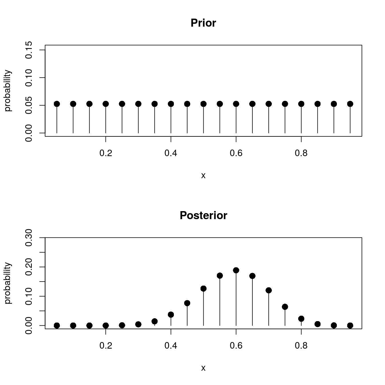
Notice the shape of the posterior. It centers around \(p = .6\), which was the sample proportion of successes. Nevertheless, other values of \(p\) could occur with high probability. We would call \(p = .6\) our maximum a-posteriori (MAP) estimate of \(p\); it is the most likely value for \(p\).
# Getting the MAP estimator for p
p[which.max(post)]
## [1] 0.6Using the posterior distribution, we can make a number of statements about the value of \(p\). For example, if we wanted to determine whether the coin is biased in favor of heads, we compute \(P(p \geq .5)\) and compare it to \(P(p < .5)\), like so:
# Is the coin biased?
sum(post[which(p >= .5)])   # Probability p >= .5
## [1] 0.8671808sum(post[which(p < .5)]) # Probability p < .5## [1] 0.1328192With \(P(p \geq .5) =\) 0.8671808, the coin is likely to be biased in favor of heads, though there is still a strong chance this may be false.
We can compute a credible interval, which is the Bayesian equivalent of a confidence interval. We will say that a \(C \times 100\)% credible interval \([a; b]\) for \(p\) is an interval such that \(P(a \leq p \leq b) = C\). I compute a (approximately) 95% credible interval for \(p\) as follows:
# Get the cdf of the posterior distribution using cumsum()
(post_cdf <- cumsum(post))
## [1] 2.142325e-11 5.695867e-08 4.733265e-06 9.562748e-05 8.848994e-04
## [6] 4.937145e-03 1.917943e-02 5.645175e-02 1.328192e-01 2.589602e-01
## [11] 4.293756e-01 6.180667e-01 7.874853e-01 9.076019e-01 9.715329e-01
## [16] 9.948018e-01 9.996236e-01 9.999972e-01 1.000000e+00# If we want the credible interval to be centered around p, we want <2.5% of
# the distribution in the lower tail, and <2.5% in the upper tail.
(a <- p[max(which(post_cdf < 0.025))])## [1] 0.35(b <- p[min(which(post_cdf > 0.975))])## [1] 0.8# What is the actual probability that a <= p <= b
sum(post[which(p >= a & p <= b)])## [1] 0.9898646The 98.99% credible interval (the closest we can get to a 95% credible interval) is [0.35, 0.8]. You can interpret this interval this interval as being the interval where there is a 98.99% chance that \(p\) lies between 0.35 and 0.8. (If this were a confidence interval, this interpretation would be wrong!)