The Burton-Pemantle Theorem
Introduction
I was recently studying the mathematical theory of composite materials, which is intimately related to homogenization theory, and came across an operator that I recognized as being of central importance in a very unrelated result: the Burton-Pemantle Theorem1. This theorem is a full description of the joint density of the edges of a uniform spanning tree on a graph. I had been aware of it for a while but it is one of those arguments that I constantly forget, so I thought it was time to write it down. There are two main reasons I find it interesting:
- to me it is a simple but concrete example of a fully discrete determinantal process, and the discrete nature means it takes less background to approach than other such processes,
- it is the natural generalization of a result first proved by Kirchoff in 1847, but almost 150 years passed before its discovery by Burton and Pemantle in the early 1990s, and
- I like uniform spanning trees.
The theorem also has a very clever proof, due to Benjamini, Lyons, Peres, and Schramm (BLPS)2, which I present below. It does seem like the kind of proof that you could only come up with once you know that the theorem is already true. However the core of the argument generalizes to other discrete determinantal processes (see the first section of Terry Tao’s notes). The BLPS proof is quite short once you understand all of the definitions, but I’ll spend some time setting it up and explaining all of the different components. I focus a lot on the physical interpretation of each piece, but try this proof if you want a shorter but purely algebraic argument.
Uniform Spanning Tree Model and the Statement of Burton-Pemantle
For the sake of simplicitly I’m only going to consider finite, undirected graphs $G = (V, E)$ in this writeup. Finite means that both $V$ and $E$ are finite sets, and while the edges initially have no direction we will soon arbitrarily assign them one. However the reason for doing so is to define an orientation on the space of edge functions for the graph, which in turn helps to carry out many computations. The choice of directions is not at all a fundamental part of the statement of the theorem. I don’t need to assume anything about the geometry of the graph, meaning specifically that the edges can form loops and there can be multiple edges between vertices, but for the sake of convenience I will assume that the graph is connected. If $G$ is not connected then the results apply to each connected component.
Recall that a spanning tree is a subset $T$ of the edge set $F$ such that the induced subgraph $(V,T)$ remains connected (the spanning part) and has no cycles (the tree part). All connected graphs obviously have at least one spanning tree, and on a finite graph the total number of spanning trees is clearly finite and is computed by the famous Kirchoff Matrix-Tree Theorem: $$ \# \textrm{ spanning trees of } G = \textrm{ reduced-det } \nabla' \nabla. $$ Here $\nabla' \nabla$ is the graph Laplacian and the reduced determinant is computed by first removing any given row and the same column from that matrix, and then computing the determinant of the resulting minor. There are several different proofs of Kirchoff’s theorem, the most common of which uses Cauchy-Binet and can be found on the Wikipedia page. Also see the proof by Lawler that is based on Wilson’s algorithm.
The uniform spanning tree model refers to exactly what it sounds like: a random spanning tree $\mathcal{T}$ chosen uniformly from the finite set of all possible spanning trees of $G$. Sometimes it is helpful to write $\mathcal{T}_G$ to emphasize the dependence on $G$. Note you don’t have to know the Matrix-Tree Theorem to make this definition, but it is nice to know that you do have a way of enumerating the set.
Of course you can also think of $\mathcal{T}$ as a random subset of the edge set $E$, and that is the approach that is most helpful for Burton-Pemantle. The theorem states:
Describing the right hand side requires some extra background which I’ll explain in the next section, but for now just think about the left hand side. It’s the probability that you’re favorite subset of edges $F$ is in a uniform spanning tree. Since $F$ can be arbitrary this means you are computing the joint density of the random edge set $\mathcal{T}$. This joint density may not be so trivial, because while all the spanning trees have an equally likely chance of being sampled this doesn’t mean that all the edges do. Even when $F$ contains only a single edge the probability that it belongs to a uniform spanning tree really depends on the overall geometry of the graph and how that edge fits into it. One can imagine that if the graph is highly connected then the probability can be quite small, but on the other hand if there’s a vertex that only has one edge connected to it then that edge is guaranteed to be in the random spanning tree. For a larger subset of edges the story can be even more complicated. Before one knows that Burton-Pemantle is true the only formula for the probability that immediately comes to mind is
$$ \mathbb{P}(F \subset \mathcal{T}) = \frac{\# \textrm{ spanning trees of } G \textrm{ that contain } F}{\# \textrm{ spanning trees of } G}, $$
and if you’re a novice in the subject it’s a bit hard to believe that a simpler formula might exist. In a sense the power of Burton-Pemantle is that you don’t have to perform the counting problem. Instead, just like in the Matrix-Tree Theorem, the determinants somewhow count everything for you. It also only requires the determinant of an $|F| \times |F|$ sized matrix, which is much smaller than the number of spanning trees. Even more miraculously, that $|F| \times |F|$ matrix is always a sub-matrix of the same matrix $\Gamma$, which we shall see in the next section is an $|E| \times |E|$ matrix determined by the geometry of the graph.
There are some quick descriptions of the matrix $\Gamma$ (see the Wikipedia entry on determinantal processes for a fast one) but I will give both a geometrical definition and some physical intuition for it. This $\Gamma$ matrix is also the key player in the Bergmann-Milton3 theory of homogenization for composites (which I learned from my colleague Ken Golden, based on his analysis4 of that theory with George Papanicolaou). Regardless of what $\Gamma$ is, if you accept the truth of the Burton-Pemantle theorem then the following must be true:
- $\det(\Gamma|_{F \times F}) = 0$ whenever $F$ is a subset of edges that contains a cycle, since of course a cycle has no chance of being in a spanning tree,
- $\det(\Gamma|_{F \times F}) = 0$ whenever $|F| > |V|-1$, since every spanning tree contains exactly $|V|-1$ edges, and consequently
- if $|F| = |V|-1$ then $\det(\Gamma|_{F \times F}) = \mathbf{1} \{ \textrm{edges of } F \textrm{ form a spanning tree } \}$, and
- for $F = \{ e \}$ one has $\det(\Gamma_{F \times F}) = \Gamma(e,e) = ||i^e||^2$, where $i^e$ is the unit current corresponding to edge $e$.
The first three facts are all obvious consequences of the identity, but the last requires some special attention and an explanation of what $i^e$ is. The identity $\Gamma(e,e) = ||i^e||^2$ is a relatively simple consequence of the way $\Gamma$ is defined, but the identity $\mathbb{P}(e \in \mathcal{T}) = ||i^e||^2$ actually comes from Kirchoff’s 1847 proof of the Matrix-Tree Theorem (see this paper for one discussion of what Kirchoff’s paper actually contains). The BLPS proof of Burton-Pemantle is recursive and uses Kirchoff’s identity to essentially end the recursion. I’ll give the precise definition of the unit current $i^e$ shortly, but intuitively it is the following: if you hook up a battery to the endpoints of the edge $e$ then currents want to flow from the positive electrode towards the negative one, and instead of only flowing through the edge $e$ it flows throughout the entire graph. Then $i^e$ is the edge function that describes the amount of current flowing through each edge.
The Transfer Current Matrix
The matrix $\Gamma$ is called the transfer current matrix, and while it is often defined in terms of star functions I prefer to give an equivalent definition that uses language with more of a calculus flavor. On the graph $G$ you have a natural gradient operator $\nabla$, defined as $$ \nabla : \mathbb{R}^V \to \mathbb{R}^E, \quad (\nabla f)(e) = f(e^+) - f(e^-). $$ Here each edge $e \in E$ is assigned an arbitrary direction, which is akin to putting an arrow on each edge, and the notation is that the arrow points away from $e^{-}$ and towards $e^{+}$. Thus $\nabla$ takes vertex functions (i.e. $\mathbb{R}^V$, the analogue of scalar functions) and returns edge functions (i.e. $\mathbb{R}^E$, the analogue of vector fields) by assigning to each edge the difference in the function’s values at the endpoints. This may seem a bit strange because we said the graph $G$ was undirected, whereas the above definition clearly requires a choice of direction for the edges. This is true, but the choice of direction is only used for setting an orientation for the edge functions $\mathbb{R}^E$. The Burton-Pemantle theorem doesn’t care which orientation you initially choose, it only matters that you do choose one and then use it consistenly thereafter. So pick an arbitrary orientation for the edges right off the start and use that in defining the $\nabla$ operator, but that orientation is only for computational purposes and has nothing to do with the discussion about spanning trees.
Now $\nabla$ is clearly a linear operator and so $\operatorname{Range}(\nabla)$ is a linear subspace of $\mathbb{R}^E$. It is a $|V|-1$ dimensional subspace since its domain is the $|V|$-dimensional space of vertex functions but has the one-dimensional space of constant vertex functions as its kernel. Of course one can project onto this subspace, and $\Gamma$ is defined as exactly this projection operator.
Clearly $\Gamma$ has an $|E| \times |E|$ matrix representation. Even though the standard matrix representation of $\nabla$ has only $-1,0,1$ in its entries, the entries for $\Gamma$ are typically much more complicated. Using the standard formula for a projection operator one would like to write $\Gamma$ as
$$ \Gamma = \nabla (\nabla' \nabla)^{-1} \nabla'. $$
Of course this is not accurate because the Laplacian $\nabla' \nabla$ is not invertible - it also has the constant functions as its kernel, but the representation is true if you remove any one column from $\nabla$ so that the remaining $|V|-1$ columns are a basis for $\operatorname{Range}(\nabla)$.
$\Gamma$ also has a natural physical interpretation beyond its mathematical definition as a projection. Graphs are often used to model electrical networks, and a central problem of such networks is to compute potentials and/or current flows on the network. To me current flow is a more natural concept than potential so I’ll explain it in that context. It’s also the description that is most relevant to $\Gamma$. The current flow problem is the following: if you connect batteries to the vertices of the network then this creates a potential difference and induces current to flow from the positive terminals to the negative ones. One wants to solve for this current given the battery configuration. The configuration itself is modeled by a function $\rho : V \to \mathbb{R}$ (i.e. $\rho \in \mathbb{R}^V$) that describes the net influx of current into each node; this can be determined solely via the batteries connected to that node. In typical physical problems the battery is only connected to a small number of vertices, meaning that $\rho$ is zero at all of the other vertices. However the induced current should be non-zero on each edge, since the electrons flow throughout the entire graph to get from the positive terminals to the negative ones. At vertices that are not connected to the batteries the total current flowing into the node should be equal to the total current flowing out, meaning that the total divergence there should be zero. If one thinks of elements of $\mathbb{R}^E$ as representing the amount of material (current, water, etc.) flowing through each edge, then one could simply define the divergence of an edge function $\theta \in \mathbb{R}^E$ to be the net amount of material flowing into and out of each vertex $v$, i.e. $$ \sum_{e \in E : e \sim v} \theta(e), $$ where $e \sim v$ means that edge $e$ is incident to vertex $v$. However there is no need to make a separate definition for this operator, since one can easily compute that $$ (\nabla' \theta)(v) = \sum_{e \in E : e \sim v} \theta(e) \textrm{ for all } v \in V, $$ where $\nabla' : \mathbb{R}^E \to \mathbb{R}^V$ is the adjoint to $\nabla$. Thus given the battery configuration as defined by $\rho,$ the current flowing along each edge is encoded by an edge function $\theta \in \mathbb{R}^E$ satisfying $$ \nabla' \theta = \rho. $$ Note the current is one such edge function satisfying the above, not the edge function, because the equation above is not enough to uniquely determine $\theta$. Indeed $\theta$ is $|E|$-dimensional while $\rho$ is $|V|$-dimensional, and since there are usually more edges than vertices in our graph this system is very underdetermined. To uniquely determine the current one invokes Ohm’s Law, which states that the current also needs to be a gradient, i.e. a member of $\operatorname{Range}(\nabla)$. Thus given $\rho$ the current flow problem means solving for $i \in \mathbb{R}^E$ that satisfies $$ \nabla’i = \rho, \quad i \in \operatorname{Range}(\nabla). $$ By writing $i = \nabla u$ for some vertex function $u \in \mathbb{R}^V$ (called the potential) this problem is usually recast as Poisson’s equation $\nabla' \nabla u = \rho$ with the potential $u$ the unknown to be solved for. Typically the solution involves some sort of Green’s function, but with the $\Gamma$ operator in hand there is another more ‘‘geometric’’ way of solving it. Indeed, as mentioned above the equation $\nabla' \theta = \rho$ admits many solutions for $\theta$, and for any such $\theta$ one can decompose it as \begin{equation}\label{eq:Gamma_decomp} \theta = \Gamma \theta + (I - \Gamma) \theta. \end{equation} The claim is that $\Gamma \theta = i$ regardless of the choice of $\theta$, and this is quick to see because:
- $\Gamma \theta \in \operatorname{Range}(\nabla)$, by definition of $\Gamma$, and
- $\nabla' \Gamma \theta = \nabla' \theta = \rho$, which follows from $I-\Gamma$ being the orthogonal projection operator onto $\operatorname{Range}(\nabla)^{\perp} = \operatorname{Ker}(\nabla')$.
The last equality is a standard fact in finite-dimensional linear algebra. Elements $\theta \in \operatorname{Ker}(\nabla')$ are called divergence free, which of course makes physical sense because it means that the net flow into each vertex is zero. Every element in $\mathbb{R}^E$ can be uniquely decomposed as a divergence free field plus a gradient, thanks to the decomposition \begin{equation}\label{eq:HH} \mathbb{R}^E = \operatorname{Range}(\nabla) \oplus \operatorname{Ker}(\nabla'). \end{equation} Recall it is a basic (and easily checked) property of linear algebra that this decomposition holds for any linear operator between finite-dimensional vector spaces. On a graph we think of edge functions as ‘‘vector fields’’, and so this is simply the Helmholtz-Hodge decomposition on a graph. Here the $\oplus$ means the direct sum of the two subspaces, and in this writeup we will only consider orthogonal direct sums, meaning that every subspace appearing in the sum is orthogonal to every other subspace in the sum. We will use this decomposition repeatedly in the final step of the proof of Burton-Pemantle, see the section on Unit Currents under Contraction.
Unit Currents
Unit currents are just currents for particular battery configurations. For each edge $e \in E$, which we recall we have given an arbitrary orientation (arrow) that points away from $e^-$ towards $e^+$, the unit current is the current flow on the graph obtained by attaching the battery to the endpoints $e^-$ and $e^+$. The precise definition is the following
This definition implies the following simple but useful results. The BLPS proof relies crucially on the fact that $\Gamma$ is a Gram matrix.
Proof of Lemma: Let $1_e \in \mathbb{R}^E$ be the indicator function of edge $e$. Then $\Gamma 1_e$ is the $e^{\textrm{th}}$ column of $\Gamma$. But by the decomposition \eqref{eq:Gamma_decomp} applied to $1_e$ and the discussion following we know that $$ \nabla' \Gamma 1_e = \nabla' 1_e = 1_{e^+} - 1_{e^-}, $$ with the last equality following by just computing the divergence of $1_e$. Thus by uniqueness of solutions to the current problem we conclude the $e^{\textrm{th}}$ column of $\Gamma$ is $i^e$. From this we also conclude that $$ \Gamma(e,f) = \langle 1_e , \Gamma 1_f \rangle = \langle 1_e, \Gamma^2 1_f \rangle = \langle \Gamma 1_e, \Gamma 1_f \rangle = \langle i^e, i^f \rangle. $$ The second and third equality use that $\Gamma$ is a self-adjoint projection. 🔲
Iterated Conditioning and the Gram Determinant
Now we’ve established what all of the central objects are and can get into the core of the BLPS proof. BLPS first notes that both $\mathbb{P}(F \subset \mathcal{T})$ and $\det(\Gamma_{F \times F})$ can be written as certain products, and then their proof concludes upon establishing the equality individual terms from each product. To match the terms correctly on each side it is convenient to label the elements of $F$, so from now on we will write $$ F = \{ e_1, e_2, \ldots, e_k \}. $$
The determinant is converted into a product relatively quickly by the following facts:
- $\Gamma$ is the Gram matrix defined by the vectors $\{ i^e : e \in E \}$, and therefore
- $\Gamma|_{F \times F}$ is the Gram matrix defined by the vectors $\{ i^e : e \in F \}$, and
- the determinant of a Gram matrix is the squared volume of the parallelotope formed by the vectors defining the matrix.
So $\det(\Gamma|_{F \times F}) = \operatorname{Vol}(\{ a_1 i^{e_1} + \ldots + a_k i^{e_k} : 0 \leq a_1, \ldots, a_k \leq 1 \})^2$. But as usual you compute the volume of a parallelotope using iterated projections onto the complementary subspaces of the span of the previously considered faces of the parallelotope, thereby obtaining
\begin{equation}\label{eq:determinant-product} \det(\Gamma|_{F \times F}) = ||P_{I_{k-1}}^{\perp} i^{e_k} ||^2 \times ||P_{I_{k-2}}^{\perp} i^{e_{k-1}}||^2 \times \ldots \times ||i^{e_1}||^2. \end{equation}
where $I_j = \operatorname{Span}\{ i^{e_1}, \ldots, i^{e_j} \}$ and $P_V^{\perp} = I - P_V$ is the orthogonal projection operator onto the subspace $V^{\perp}$.
Now put \eqref{eq:determinant-product} aside for a minute and go back to $\mathbb{P}(F \subset \mathcal{T})$. It can be computed by iteratively conditioning, meaning
$$
\begin{eqnarray*}
\mathbb{P}(e_1, e_2, \ldots, e_k \in \mathcal{T}) &=& \mathbb{P}(e_2, \ldots, e_k \in \mathcal{T} | e_1 \in \mathcal{T}) \mathbb{P}(e_1 \in \mathcal{T}) \\\
&=& \vdots \\\
&=& \mathbb{P}(e_k \in \mathcal{T} | e_1, \ldots, e_{k-1} \in \mathcal{T}) \ldots \mathbb{P}(e_2 \in \mathcal{T} | e_1 \in \mathcal{T}) \mathbb{P}(e_1 \in \mathcal{T}).
\end{eqnarray*}
$$
For these terms we finally use the *uniform* part of the model and make the following observation:
\begin{equation}\label{eq:contraction-identity}
\mathcal{L}(\mathcal{T}_G | e \in \mathcal{T}_G) = \mathcal{L}(\mathcal{T}_{G / e}),
\end{equation}
where $\mathcal{L}$ denotes the law of the random objects (the left hand side being the law under conditioning) and $G / e$ is the contracted graph obtained by identifying the endpoints of edge $e$ as the same vertex.
Equation \eqref{eq:contraction-identity} should be fairly intuitive: if you start with a spanning tree that contains $e$ and then contract the graph along $e$ then what remains is a spanning tree on $G / e$. And of course when you condition a uniform random variable it remains a uniform random variable, so the probabilities are preserved exactly as described. Using this fact in the above equation we get \begin{equation}\label{eq:iterated-condition} \mathbb{P}(e_1, \ldots, e_k \in \mathcal{T}_G) = \mathbb{P}(e_k \in \mathcal{T}_{G_{k-1}}) \mathbb{P}(e_{k-1} \in \mathcal{T}_{G_{k-2}}) \ldots \mathbb{P}(e_1 \in \mathcal{T}_G), \end{equation} where $G_i$ is the contracted graph $G_i = G \backslash \{ e_1, \ldots, e_i \}$. This graph can be obtained by contracting iteratively or all at once, it doesn’t matter how you do it.
Now when you compare \eqref{eq:determinant-product} and \eqref{eq:iterated-condition} you see the obvious strategy for finishing the proof of Burton-Pemantle: just prove that $$ ||P_{I_{k-1}}^{\perp} i^{e_k}||^2 = \mathbb{P}(e_k \in \mathcal{T}_{G_{k-1}}), ||P_{I_{k-2}}^{\perp} i^{e_{k-1}} ||^2 = \mathbb{P}(e_{k-1} \in \mathcal{T}_{G_{k-2}}), \ldots, $$ and $||i^{e_1}||^2 = \mathbb{P}(e_1 \in \mathcal{T})$. Of course you should first have some sense that all of these equalities are actually true, but we already know that $$ ||i^{e_1}||^2 = \mathbb{P}(e_1 \in \mathcal{T}). $$ from the previously mentioned Kirchoff theorem for single edge marginals of the uniform spanning tree. We will just accept this result, but you can find a description of it in the summary paper on Kirchoff’s theorem. This leaves us to prove the remaining $k-1$ identities, but once you know Kirchoff’s result they start to look more plausible. For example, for $j=2$ we need to show $$ ||P_{I_1}^{\perp} i^{e_2}||^2 = \mathbb{P}(e_2 \in \mathcal{T}_{G_1}), $$ which, by untangling the definitions, can be rewritten as $$ ||(I - P_{i^{e_1}}) i^{e_2}||^2 = \mathbb{P}(e_2 \in \mathcal{T}_{G / e_1}). $$ Here $P_{i^{e_1}}$ is the orthogonal projection onto $\operatorname{Span} \{ i^{e_1} \}$. By the Kirchoff theorem again the right hand side can be replaced by the squared norm of a unit current, which converts the desired equality into $$ ||(I - P_{i^{e_1}}) i^{e_2}_G||^2 = ||i^{e_2}_{G / e_1}||^2. $$ Note that we’ve now added subscripts to the unit currents to keep track of which graph they are coming from. In short, thanks again to the Kirchoff theorem proving the $j=2$ case requires showing that the norm of the unit current for $e_2$ on the contracted graph $G / e_1$ is equal to the norm of the projection of the unit current for $e_2$ on the original graph $G$.
Of course if you believe that this property is true then you should also believe it is true on arbitrary graphs and for arbitrary pairs of edges, since we haven’t assumed anything about them in the preceding discussion. Thus the desired identity should rely on some general result about how unit currents behave under contraction of a graph, and the BLPS proof is completed by working out the precise statement. This is done in the next section, and one thing we’ll see is that the general statement is actually an identity between the vectors, not just their norms.
The other observation to make is that if we prove this more general statement, which covers the $j=2$ case of the identities above, then we can iterate it to also prove the $j \geq 3$ identities. This would complete the proof of Burton-Pemantle. The reason that we can iterate is because both projection and contraction can be done either in steps or all at once, but either way produces identical results. Hopefully this is intuitive enough, but the algebra can be worked out quite easily if you want to convince yourself further.
Unit Currents under Contraction
As promised we now study how unit currents behave under contraction. This is a simple but fundamental result, and the argument here is just a rewriting of equations (4.3) and (4.4) in the book by Lyons and Peres.
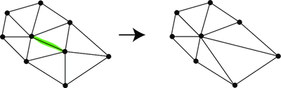
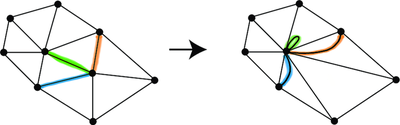
The proof is an analysis of the gradient operators $\nabla_G$ and $\nabla_{G / e}$ and their adjoints. In the remainder we always write the subscript to denote the dependence on the graph. The proof uses that the Helmholtz-Hodge decomposition \eqref{eq:HH} holds on any graph, and in particular on both $G$ and the contracted graph $G / e_1$. To make the argument conceptually easier I prefer to consider contraction in a way that preserves the edge set. Specifically this means that $e_1$ is contracted into a loop, and the other edges incident to the endpoints of $e_1$ now become multi-edges. The figure below shows an example.
With this convention the contracted graph $G / e_1$ has the same edge set as $G$, and since the presence of loops and multi-edges doesn’t complicate the definition of the gradient operator this means that the space of edge functions can be decomposed in two different ways:
\begin{equation}\label{eq:HH-double}
\mathbb{R}^E = \operatorname{Range}(\nabla_G) \oplus \operatorname{Ker}(\nabla_G') = \operatorname{Range}(\nabla_{G / e_1}) \oplus \operatorname{Ker}(\nabla_{G / e_1}').
\end{equation}
BLPS proves the lemma by deducing the relation between the two decompositions. They show
\begin{eqnarray}
\operatorname{Range}(\nabla_G) &=& \operatorname{Range}(\nabla_{G / e_1}) \oplus \operatorname{Span}(i^{e_1}_G), \label{eq:HH-double-1} \\\
\operatorname{Ker}(\nabla_{G / e_1}') &=& \operatorname{Ker}(\nabla_G') \oplus \operatorname{Span}(i^{e_1}_G), \label{eq:HH-double-2}
\end{eqnarray}
which essentially says that under contraction the subspace spanned by the unit current $i^{e_1}$ moves from being in the gradient space in $G$ to being in the orthogonal complement of the gradient space in $G / e_1$. This is intuitively clear if you know that the orthogonal complement to gradients is the cycle space. Under contraction the single edge $e_1$ becomes a cycle on its own, which is the reason for the decomposition above. The proof is in the pop down text below, so take a look if you wish (just click on the arrow), but if you don’t want to spoil the flow you can just accept it as fact and move on.
Proof of \eqref{eq:HH-double-1}-\eqref{eq:HH-double-2}
If you accept that $\operatorname{Ker}(\nabla_G')$ is the cycle space of the graph (for any $G$), then stare at the picture above until you convince yourself that the cycles in the original graph remain cycles in the contracted graph, except that the edge $e_1$ becomes a cycle on its own. Therefore $$ \operatorname{Ker}(\nabla_{G / e_1}') = \operatorname{Ker}(\nabla_G) + \operatorname{Span} \{ 1_{e_1} \}, $$ where $1_{e_1}$ is the indicator function of the edge $e_1$. The right hand side is a sum of subspaces but is not orthogonal. To make it orthogonal simply project out the part of $1_{e_1}$ inside of $\operatorname{Ker}(\nabla_G)$; this is achieved by the projection $I-\Gamma$. What is left is precisely $\Gamma 1_{e_1} = i^{e_1}$, which proves \eqref{eq:HH-double-2}. Then \eqref{eq:HH-double-1} follows from \eqref{eq:HH-double-2} and \eqref{eq:HH-double}.
A quick argument that $\operatorname{Ker}(\nabla_G')$ is the cycle space is the following: you already know $\operatorname{Ker}(\nabla_G') = \operatorname{Range}(\nabla_G)^{\perp}$, and from this the cycle space comes into play by recalling that an edge function is a gradient iff it sums to zero around all cycles of the graph (with edge orientation taken into account in the proper way). 🔲
Assuming this fact we are now able to prove the lemma.
Proof of Lemma: Using \eqref{eq:HH-double-1} and the fact that the unit current $i_G^{e_2}$ is in $\operatorname{Range}(\nabla_G)$ (by definition of unit current), this means there is a $\psi \in \operatorname{Range}(\nabla_{G / e_1})$ and $c \in \mathbb{R}$ such that $$ i^{e_2}_G = \psi + c i^{e_1}. $$ Thus $(I - P_{i^{e_1}}) i^{e_2}_G = \psi$, and we want to show that $\psi = i^{e_2}_{G / e_1}$. It is enough to show that $$\nabla_{G / e_1}' \psi = 1_{e_2^+} - 1_{e_2^-},$$ since $i_{G / e_1}^{e _2 }$ is the unique element of $\operatorname{Range}(\nabla_{G / e_1})$ with this property. But this follows by applying the divergence operator to both sides of the last equation, i.e. $$ 1_{e_2^+} - 1_{e_2^-} = \nabla_G' i_G^{e_2} = \nabla_{G / e_1}' i^{e_2}_G = \nabla_{G / e_1}' (\psi + c i^{e_1}_G) = \nabla_{G / e_1}' \psi. $$ The second and last equality are explained by $$ (\nabla_{G / e}' \theta)(v) = (\nabla_G' \theta)(v) \textrm{ for } v \not \in \{ e^+, e^- \}, $$ which holds because contraction does not affect the divergence away from the contracted edge, while at the endpoints of the contracted edge one has $$ (\nabla_{G / e}' \theta)(e^+) = (\nabla_{G / e}' \theta)(e^-) = (\nabla_G' \theta)(e^+) + (\nabla_G' \theta)(e^-). $$ Together with the defining properties of $i_G^{e_1}$ and $i_G^{e_2}$ these identities show that $$ \nabla_{G / e_1}' i_G^{e_1} = 0, \quad \nabla_G' i_G^{e_2} = \nabla_{G / e_1}' i^{e_2}_G. $$ The last equality uses that $e_1$ and $e_2$ are distinct and hence share at most one common endpoint vertex. This completes the proof. 🔲
Summary of the Proof
So in short, the steps of the proof are the following:
- Use repeated conditioning and the Gram identity to write both the desired probability and the determinant as a product of terms.
- Show equality of individual terms in the product, essentially by an inductive argument. This step is fundamental and is based on the analysis of how unit currents behave under contraction of edges on a graph.
- Appeal to Kirchoff’s Matrix Tree Theorem as the base step of the induction.
The hardest part of the proof is certainly the analysis of how unit currents behave under contraction. If you are still somewhat unclear you may wish to read that section again. For myself equation \eqref{eq:unit-current-contraction} somehow becomes clear by simply staring at the picture of the contracted graph for a while.
The Weighted Spanning Tree Model
There is an extended version of the Burton-Pemantle theorem that holds for spanning trees with weights. In this setting one attaches resistances $r : E \to (0, \infty)$ to the edges and defines the weight of each spanning tree $T$ of $G = (V,E)$ to be \begin{equation}\label{eq:weighted-model} w(T) = \prod_{e \in T} r(e)^{-1} = \prod_{e \in T} c(e), \end{equation} where we let $c(e) = r(e)^{-1}$ be the conductances. The weighted uniform spanning tree corresponding to these conductances is the probability measure on spanning trees defined by $$ \mathbb{P}_c(T) = \frac{w(T)}{\sum_T w(T)}. $$ Kirchoff’s Matrix-Tree Theorem can be extended (with no real work) to show that $$ \sum_T w(T) = \textrm{reduced-det } \nabla' c \nabla, $$ where in the $c$ in the middle is regarded as a multiplication operator, i.e. an $|E| \times |E|$ diagonal matrix with diagonal entries $c(e)$. Under $\mathbb{P}_c$ only the matrix $\Gamma$ changes in the Burton-Pemantle Theorem. In the weighted case it gets replaced by a matrix $\Gamma_c$, which can be equivalently defined as:
- again the $|E| \times |E|$ matrix whose columns are the unit currents $i^{e_1}$, except that now the unit currents are the unique elements of $\operatorname{Range}(c \nabla)$ whose divergence satisfies $\nabla' i^{e_1} = 1_{e_1^+} - 1_{e_1^-}$,
- the orthogonal projection operator onto $\operatorname{Range}(c \nabla)$ in the weighted inner product $$ \langle \theta, \psi \rangle_r = \sum_{e \in E} r(e) \theta(e) \psi(e). $$
The appearance of the conductances $c$ in $\operatorname{Range}(c \nabla)$ again comes again from Ohm’s Law: $\nabla v = i r$ where $v$ is the potential/voltage. If you’re working out $\Gamma_c$ numerically it is useful to remember that $\Gamma_c$ will not be symmetric when expressed in the standard basis, because it is only self-adjoint in the weighted inner product $\langle \cdot, \cdot \rangle_r$. That self-adjointness however implies that the matrix $r \Gamma_c$ is symmetric when expressed in the standard basis.
Given these changes in the setup and the statement of the theorem, the elements of the proof change essentially mutatis mutandis. Specifically:
-
The contraction identity \eqref{eq:contraction-identity} and its consequence \eqref{eq:iterated-condition} is easily seen to be replaced by $$ \mathbb{P}_c(e_1, \ldots, e_k \in \mathcal{T}_G) = \mathbb{P}_c(e_k \in \mathcal{T}_{G_{k-1}}) \mathbb{P}_c(e_{k-1} \in \mathcal{T}_{G_{k-2}}) \ldots \mathbb{P}_c(e_1 \in \mathcal{T}_G), $$ which follows because the weight of each tree in \eqref{eq:weighted-model} has a product structure.
-
The matrix $\Gamma_c$ is still a Gram matrix, although now one must be careful to write it as $\Gamma_c = \Gamma_c^* \Gamma_c$ where $\Gamma_c^*$ denotes adjoint in the weighted inner product. The fundamental property that the determinant of a Gram matrix is the squared volume of the parallelotope formed by the vectors defining the matrix is still true, except that volume is now computed with respect to the weighted inner product (which in turn defines lengths). The iterated projections formula \eqref{eq:determinant-product} is still true, except that now projections and lengths are computed in the weighted inner product. In many ways the use of the Gram determinant is better explained in the Lyons and Peres book book than in the exposition here, since the argument there essentially *proves* the iterated projections formula for Gram determinants, whereas here we simply invoke it.
-
Equation \eqref{eq:unit-current-contraction} for the behavior of unit currents under contraction remains true, except on the right hand side the projection takes place in the weighted inner product $\langle \cdot, \cdot \rangle_r$. The Hodge decomposition \eqref{eq:HH} that is fundamental in the proof is replaced by $$ \mathbb{R}^E = \operatorname{Range}(c \nabla) \oplus_r \operatorname{Ker}(\nabla'), $$ where the symbol $\oplus_r$ means ‘‘direct sum of orthogonal subspaces in the weighted inner product’’. It is straightforward to check that the two subspaces are orthogonal in this inner product; indeed this is the fundamental fact in using the transfer current matrix $\Gamma_c$ to solve for currents in the Poisson equation.
-
Burton R., & Pemantle R. (1993). Local Characteristics, Entropy and Limit Theorems for Spanning Trees and Domino Tilings Via Transfer-Impedances. The Annals of Probability, 21(3), 1329–1371. Online Journal ↩︎
-
Benjamini I., Lyons R., Peres Y., & Schramm O. (2001). Uniform Spanning Forests. The Annals of Probability, 29(1), 1-65. Online Journal. See also the version of this proof in Hough, Krishnapur, Peres, and Virag, and the book Probability on Trees and Networks by Lyons and Peres. ↩︎
-
There are many sources for the Bergmann-Milton theory. See the textbook by my colleague Graeme Milton for a comprehensive review: Milton G. (2002). The Theory of Composites. Cambridge Monographs on Applied and Computational Mathematics, Cambridge: Cambridge University Press. Online Version ↩︎
-
Golden K., & Papanicolaou G. (1983). Bounds for effective parameters of heterogeneous media by analytic continuation. Communications in Mathematical Physics, 90(4), 473-491. Online Journal ↩︎