DYNAMIC VISUALIZATION OF SUMS OF POSITIVE INTEGERS AND THEIR SQUARES

The formulas for the sum of the first n positive integers and for the sum of the squares of the first n integers are useful in calculus for finding definite integrals of

f(x)=x and f(x)=x² directly from their definition, and in linear algebra for finding how many arithmetic operations are needed to solve a system of n linear equations

in n unknowns by the method of Gaussian elimination, and how many are required when just the "right-hand side" is changed. The animations on this page visualize a

method for obtaining both of these formulas, and their generalization to arbitrary powers, in a unified manner. When viewed dynamically, they give a visual meaning

to the integral-derivative relationship between F(x)=x² and f(x)=2x, and between F(x)=x³ and f(x)=3x². The visualizations express a binomial expansion, also

used to derive the power rule for derivatives, and emphasize the duality and symmetry between differentiation and integration. The derivations involve collapsing sums,

and foreshadow the connection between rates of change and geometric boundaries made systematic in the various Stokes' theorems of multivariable calculus.

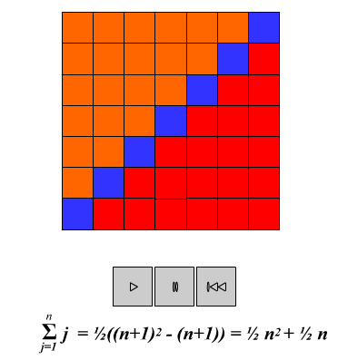
The formulas visualized at successive stages of the animation are:

The general formula illustrated is:

We then solve for the sum of the whole numbers less than or equal to n.

The general formula illustrated is:

The final formula

can be derived in several other ways (e.g., interpolation) and proven true for all n by induction. It may be used to compute the integrals

directly. This shows that both the 1/2 in these integration formulae and the 2 in the differentiation formula

come from a common source, the second entry of the second row of Pascal's triangle.

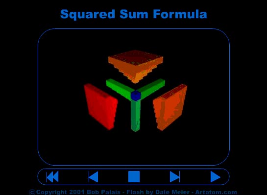
SUM OF THE SQUARES OF THE FIRST N NATURAL NUMBERS (N=6)

The formulas visualized at successive stages of the animation are:

The general formula illustrated is:

Substituting the formula for the sum of whole numbers less than or equal to n, we then solve for the sum of the squares of the whole numbers less than or equal to n.

The general formula illustrated is:

where we have used

.

The final formula

can be derived in several other ways (e.g., interpolation) and proven true for all n by induction. It may be used to compute the integrals

directly. This shows that both the 1/3 in these integration formulae and the 3 in the differentiation formula

come from a common source, the second entry of the third row of Pascal's triangle.

An analogous derivation can be made for any power, m. The sum from j=1 to n of j^m is a polynomial of degree m+1 in n. The coefficient of n^m+1 is 1/(m+1), and the constant coefficient is zero.

The coefficient n^m+1-k is B(k)C(m+1,k)/(m+1), where B(k) is the kth Bernoulli number, and C(n,k) is a binomial coefficient.

(See: http://en.wikipedia.org/wiki/Bernoulli_number#Sum_of_powers and http://en.wikipedia.org/wiki/Binomial_coefficient for details.)

THE COMPUTATIONAL COMPLEXITY OF SOLVING N EQUATIONS IN N UNKNOWNS BY GAUSSIAN ELIMINATION

These sums are also important in understanding the computational complexity of solving n equations in n unknowns by Gaussian elimination. This method replaces

the original set of equations with an equivalent (having the same solutions) but simpler set by inductively eliminating the first remaining variable from all but the first

remaining equation (reorderings of equations and/or variables may be required, or recommended to maintain stability) until either no variables or equations remain.

The elimination is performed by subtracting a multiple of the first remaining equation from each of the other remaining equations so that the resulting coefficient of the

variable in question becomes zero. In the simplest case, we first eliminate the first variable from n-1 remaining equations . To do this we subtract the appropriate

multiple of the coefficient of the n-1 remaining variables in the first equation from the corresponding variable in the n-1 remaining equations. This involves n-1

multipliers, and(n-1) ² multiplications and subtractions. By the same reasoning, to eliminate the second variable from n-2 equations involves n-2 multipliers

and (n-2) ² multiplications and subtractions, until we eliminate the n-1st variable from 1 equation with 1 multiplier, for one multiplication and subtraction.

So elimination requires

multiplications and subtractions (additions). There are

coefficients remaining in the resulting equivalent system of equations, for n variables in the first, n-1 in the second, etc.

multipliers were found by the same number of divisions (but no multiplications or subtractions were needed since we already knew the result would be zero! When

programming this algorithm, the multipliers are typically stored where those zeroes would be. So far we have only mentioned the elimination aspect, but what about

solving the equations? The reason we have done so is to emphasize that these tasks may be separated and that to solve the equations with the original right-hand side or

any other involves the same work. We must perform the sameoperations on both sides of each equation to preserve equality, so as we subtract multiples of one

equation from another, we must also subtract the same multiple of the corresponding right-hand side from the other right-hand side. Regardless of what initial right-

hand side we are considering, we just perform the

multiplications and subtractions, one for each multiplier involved in the elimination, to obtain the corresponding right-hand side in the equivalent eliminated equations.

Finally, we take advantage of their simpler form to solve for the unknowns. The last equation of this system had only one unknown, and we can solve one equation in

one unknown by dividing by its (non-zero) coefficient. The next-to-last equation had two unknowns, including the last variable, which is now known, so it now

becomes one equation in one unknown. We solve for the second-to-last variable by subtracting the last variable times its coefficient in the second-to-last equation from

the right-hand side of that equation, and divide by the (non-zero) coefficient of the second-to-last variable, and so on. This process again involves

multiplications and subtractions, plus n divisions.

The upshot of this analysis is best understood by imagining a linear system of equations arising from a three-dimensional model involving 100 grid points in each

direction, or 1 million variables. Solving such a system by elimination could involve about 10 ¹⁸ arithmetic operations! That's about a billion seconds or thirty

years at a billion operations per second. In contrast, once the multipliers and resulting eliminated system are known, the system can be solved for any given right-hand

side with only 10 ¹² additional operations, about one thousand seconds or twenty minutes, at the same rate - and about a million times faster than solving the

system again from scratch! We'll discuss how to approach these difficulties by using alternative methods or taking advantage of any special structure of the matrix;

why elimination can fail to work even when it doesn't take too long, and how to fix it, elsewhere.