Consider the following autonomous differential equation: \begin{equation} \label{} y' = y(y-2). \label{eqn-autonomous-example}\tag{3.1.2} \end{equation} Notice that the two constant functions \(y(x)=0\text{,}\) and \(y(x)=2\) are solutions to equation (3.1.2). In fact any time you have an autonomous equation, any constant function which makes the right hand side of the equation zero will be a solution. This is because constant functions have derivative zero. Thus as long as this constant value of \(y\) is a root of the right hand side, then that particular constant function will satisfy the equation. Notice that other constant functions such as \(y(x)=1\) and \(y(x)=3\) are not solutions of equation (3.1.2), because \(y' = 1(1-2)=-1 \ne 0\) and \(y' = 3(3-2) = 1 \ne 0\) respectively.

So the critical points of equation (3.1.2) are \(0\) and \(2\text{.}\)

So the equilibrium solutions of equation (3.1.2), are \(y=0\) and \(y=2\text{.}\) Something in equilibrium, is something that has settled and does not change with time, i.e. is contant.

Example3.1.4Another Phase Diagram

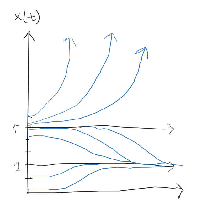
Create a phase diagram and plot several solution curves by hand for the differential equation: \begin{equation*} \frac{dx}{dt} = x^3 - 7x^2 + 10x \end{equation*}

We factor the right hand side to find the critical points and hence equilibrium solutions. \begin{align*} x^3 - 7x^2 + 10x \amp = 0\\ x(x^2 -7x + 10) \amp = 0\\ x(x-2)(x-5) \amp = 0 \end{align*} The critical points are \(0,2,5\text{,}\) and thus the equilibrium solutions are \(x=0, x=2\) and \(x=5\text{.}\)

Our earlier population model suffered from the fact that eventually the population would “blow up” and grow at unrealistic rates. This was due to the fact that the solution involved an exponential function. Recall the model and solution: \begin{equation*} \frac{dP}{dt} = kP, \: P(0)=P_0 \qquad P(t) = P_0 e^{kt}. \end{equation*}

Bacteria in a petri dish can't reproduce forever because they eventually run out of food and space. In our previous population model, the constant of proportionality was actually the birth rate minus the death rate: \(k = \beta - \delta\text{,}\) where \(k\) and therefore also \(\beta\) and \(\delta\) have units of 1/time.

To make our model more realistic, we need the birth rate to taper off as the population reaches a certain number or size. Perhaps the simplest way to accomplish this is to have it decrease linearly with population size. \begin{equation*} \beta(P) = \beta_0 - \beta_1 P \end{equation*} For this to make sense in the original equation, \(\beta_0\) must have units of 1/time, and \(\beta_1\) must have units of 1/(population\(\cdot\)time). Let's incorporate this new, decreasing birth rate into the original population model.

\begin{align*} \dfrac{dP}{dt} \amp = [(\beta_0 - \beta_1 P) - \delta]P\\ \amp = P[(\beta_0 - \delta) - \beta_1 P]\\ \amp= \beta_1 P \left[ \dfrac{\beta_0 - \delta}{\beta_1} - P \right] \end{align*}

In order to get a simple, easy to remember equation, let's let \(k = \beta_1\) and \(M = \frac{\beta_0 - \delta}{\beta_1}\text{.}\) \begin{equation} \boxed{\dfrac{dP}{dt} = k P ( M - P )} \label{eqn-logistic-model}\tag{3.1.3} \end{equation}

Notice that \(M\) has units of population. We have specifically written equation (3.1.3), in the form at the bottom of the derivation because \(M\) has a special meaning, it is the carrying capacity of the population.

Notice that equation (3.1.3) is autonomous, so we know how to go about solving it. However, before we solve the logistic model, let's refresh our memory of solving integrals via partial fractions, because we will need to use this when solving the logistic model. Let's solve a simplified version of the logistic model, with \(k=1\) and \(M=1\text{.}\)