My overarching research goal is to bring the advanced tools of mathematics to bare on relevant real world problems bringing new perspectives to some fields, improving general scientific understanding, and fostering new methods for prediction and analysis. I also believe that such pursuits create a positive feedback into mathematics, inspiring new ways of thinking, motivating new mathematical developments, and providing a bed rock to test such developments. This positive feedback between mathematics, applied problems, and experiment guides my research philosophy. Perhaps there is a nice mathematical idea for which we would seek to find a problem to which it may apply, maybe it’s a pressing real world problem that needs innovative approaches, or it is just an interesting data set or experimental result that can spawn new ideas and innovations. Any of these can serve as a starting point, mid point or end point but their interplay is key. To that end, I believe in a sort of kitchen sink approach, not in the sense that we indiscriminately try every thing until something seems to stick, but that we don’t limit our set of tools, approaches, starting points, or motivation. We should work in an interdisciplinary way seeking collaboration with those who can offer knowledge, skills, or resources that may move a piece of work forward perhaps gaining new insight and skills along the way. I believe the real benefit of working in applied mathematics is the freedom to truly be interdisciplinary and not locked into one specific way of thinking. I also believe, when possible, an attempt should be made to accelerate research to application beyond initial publication, something I have enjoyed doing at the Joint Center for Satellite Data Assimilation these last few years.

Throughout my career, my main scientific interest has been focused on Earth’s climate in some way or another and more recently on data assimilation aimed at improving weather prediction, something I consider important as extreme weather becomes more common. Both areas of research provide many opportunities to experience an interdisciplinary feed back. As an undergraduate and continuing into graduate school I worked on problems involving sea ice utilizing campus labs to design experimental methods I was fortunate to employ in Arctic and Antarctic field campaigns. I have been involved in research which applies: percolation theory to electrical and fluid transport through the porous microstructure of sea ice [15],[14]; inversion theory to problems in remote sensing [29]; graph theory to melt pond evolution [1]; and homogenization theory to ocean wave dynamics in the marginal ice zones (MIZ) of the Arctic and Antarctic [31]. That work was been guided by the fact that sea ice may be thought of as a composite material over multiple scales and was inspired by in person observation of waves propagating through the MIZ in the Antarctic.

As a postdoc, I began working with larger data sets primarily through the lens of Data Assimilation (DA) and Statistical or Machine Learning techniques. Working with others from across the globe we: developed new techniques allowing the application of the Ensemble Kalman Filter (EnKF) to models which use non-conservative adaptive mesh solvers [32] (motivated by a lagrangian sea ice model); employed new metrics using boundary preserving diffeomorphisims to calibrate a sea ice model [38] (that explicitly models leads) using SAR satellite imagery [16]; applied ensemble smoothing techniques with an age stratified SEIR model to study the spread of SARS-CoV-2 (the virus that causes COVID-19) obtaining continuous time series of the basic reproductive number R₀ which, can be used to evaluate successes and failures of various mitigation strategies [7]; extended the previously mentioned model and DA method to a multi-group population model to study disparities in the impact of the pandemic on different racial/ethnic groups [9]. The ESMDA method proved so powerful in accurately estimating time dependent parameters, we later applied it to a reduced order model of the polar vortex with two main controlling parameters, h (representing perturbations from topography) and λ (representing the thermal gradients) [34]. The data assimilated came from the ECMWF ERA 5 reanalysis set and we found the reduced order model, when parameters were time dependent, could reproduce more complex behavior of the polar vortex and found signatures of sudden stratospheric warming (SSW) events in the state and parameter analyses. I was also involved in some work employing Generative Adversarial Networks (GANs) trained on images of melt ponds on Arctic sea ice to produce realistic meltpond geometries for use in sea ice modeling; and studying sea ice microstructure through the lens of topological data analysis [30].

While there is inherent value in all research, the value of that work can be multiplied if it can be readily applied. When working in the field of DA I noticed a divide between those doing fundamental research and those applying DA in weather and climate science. One of the primary reasons for this divide are the systems used by each group to do the research. Mathematicians typically stick to toy models and ideal situations with code written in Python or Matlab for demonstrations of new ideas. While these are good for initial development this makes adoption of new ideas by the scientific community at large slow and difficult. Large scale models are complex, legacy objects which are difficult to adapt for new ideas and can require full time employees to implement anything novel, even just for testing. This seems a shame in a field where rapid developments are taking place that could benefit the scientific community at large. This has been recognized by in atmospheric and climate science and is being addressed through the development of the Joint Effort for Data assimilation Integration (JEDI) system. JEDI is funded by NASA, NOAA, The Navy, USAF, and UK Met Office and is a generic Data Assimilation system meant to be used with each partner’s model and observations. JEDI will be the operational system for each of those agencies in the very near future. To facilitate that, JEDI is designed in such a way that any model with an JEDI interface has access to the whole system, so that when a new development is added it is immediately available. It is for this reason I applied for a position at the Joint Center for Satellite Data Assimilation (JCSDA) in late 2021. I wanted to gain experience closer to operational settings and hopefully directly contribute new innovations. One such new innovation I was tasked to add to JEDI is a Hybrid Differential Tangent Linear Model (HTLM) developed in [25] which showed promise in improving 4d-Var assimilations and allowing for the use of 4d-Var with new model physics without the costly updating of the traditional tangent linear model. The HTLM at it’s core uses an ensemble of nonlinear model runs to correct linear model trajectories when the linear model itself is missing linearized physics or is otherwise incomplete. After its addition to JEDI, the HTLM is being used with NASA’s GEOS model for atmospheric composition experiments, NOAA GFS for 4d-Var experiments with metrology, and with the Sea Ice and Ocean Coupled Assimilation (SOCA) system in JEDI to enable 4d-Var experiments there. I think this is a success story where a new innovation was made readily available to the community at large and as a result was quickly adoptable enabling new science to be done. This is something I would hope to continue to be able to do in my research when possible, I could imagine developing and testing new ideas in DA directly in JEDI and if successful then making them immediately available to the community at large as a result. While the scientific community can benefit from innovations added to JEDI, researchers can benefit from development in systems like JEDI as well. In addition to Lorenz 95 and Quasi-Geostrophic toy models, JEDI provides access to the kinds of large scale models that are difficult to develop and test with, it opens the door to doing fundamental research in a setting otherwise very difficult to work in. Not can only new DA methods be tested with real complex atmospheric models, new ideas in modeling are made easier to test and develop as well. One could add a new physical parameterization to MPAS for example and use JEDI to run it, estimate parameters, or evaluate forecast scores with and without DA. This is especially relevant for research toward improving extreme weather prediction, something I think that should be considered important climate research. However even with all of these benefits, it would be nice to extend the utility of systems like JEDI to more basic and developmental research. I would love to develop a tool which allowed researchers to prototype new ideas in climate science, perhaps novel ODE/PDE reduced order models, a new parameterization of a physical phenomena, an ecological, epidemiological, or migration model in a simple way and generate a JEDI interface for those models. This would aid in running simulations on HPC environments as well as connect new models to the DA Algorithms, observations operators, and data ingest tools already available in JEDI. I would also love to see more DA methods aimed at developmental models included in JEDI like ESMDA or novel particle filters, for example. There are also existing ideas that could easily be added, tested and iterated upon such as Feature Calibration and Alignment (FCA) analysis [23] which aligns coherent structures as part the analysis. I also believe there is opportunity for development in the Community Radiative Transfer Model (CRTM), particularly with respect to sea ice microwave emissivity, something that could benefit from an experimental component. All in all, I believe there is a real novel opportunity to create a research program that drives new fundamental innovations with an aim of accelerating their application as a core mission objective. The pursuit of that objective strengthens the interdisciplinary feedback that is so beneficial to applied mathematics and science as whole.

Data Assimilation and Ensemble Methods

Ensemble Methods for Parameter Estimation and General Reanalysis

Ensemble smoother techniques can be derived by assuming a perfect forward model.

(1)

In general, x is the realization of model parameters, and y consists of the uniquely predicted measurements resulting from the parameters x through the model operator g(x). The vector y then consists of the predicted measurements given some model error, e. To solve the inverse problem, it is efficient to frame it into an equation using Bayes’ theorem:

(2)

Equation ( 2) represents the so-called smoothing problem, which can be approximated using ensemble methods. In practice this problem can be solved using an iterative ensemble smoothing method called an ensemble smoothing with multiple data assimilation (ESMDA). The method, which is similar to an ensemble smoother, solves the parameter-estimation problem and is formally derived from the Bayesian formulation using a tempering procedure [37]. What separates this method from other similar methods is that it approximates the posterior recursively, gradually introducing information to alleviate the impact of any nonlinear approximations. After updating through to the last time step, it begins the assimilation process over again - resampling the vector of perturbed observations, which reduces sampling error [6]. The general steps can be described simply. (1) Sample a large ensemble of the parameters you wish to estimate assigning uncertainty to each. (2) Integrate the ensemble of model realizations forward in time to obtain a prior ensemble prediction. (3) Compute the posterior of the ensemble of parameters using the difference between predicted states and observations with the correlations between those parameters and predicted states. (4) Integrate the ensemble of updated model realizations forward in time and repeat for the number of ESMDA steps chosen. After the cycle is completed the ensemble mean of parameters are considered optimal as well as the mean of model predictions arising from the ensemble of parameters. One also obtains a measure of uncertainty through the spread in the parameters as well.

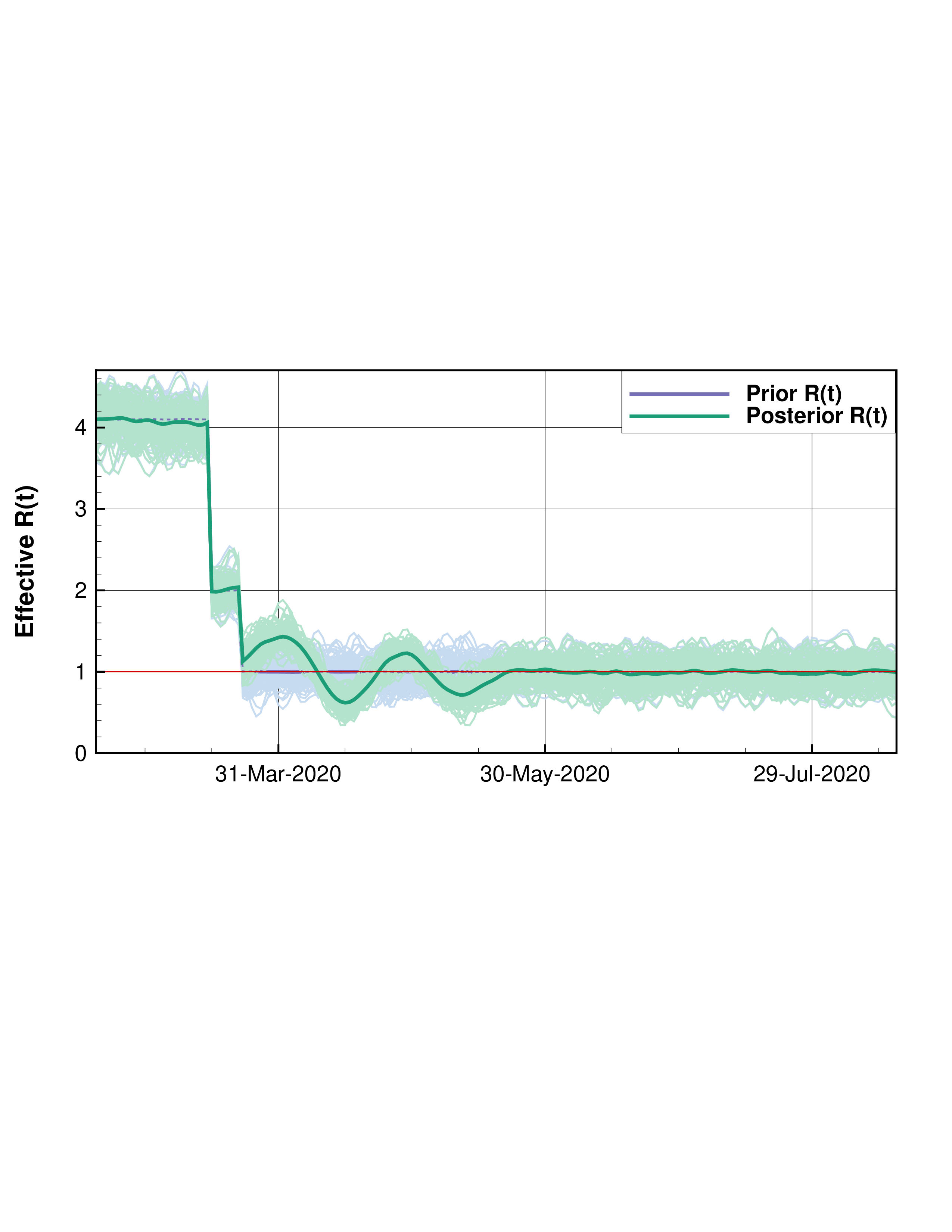
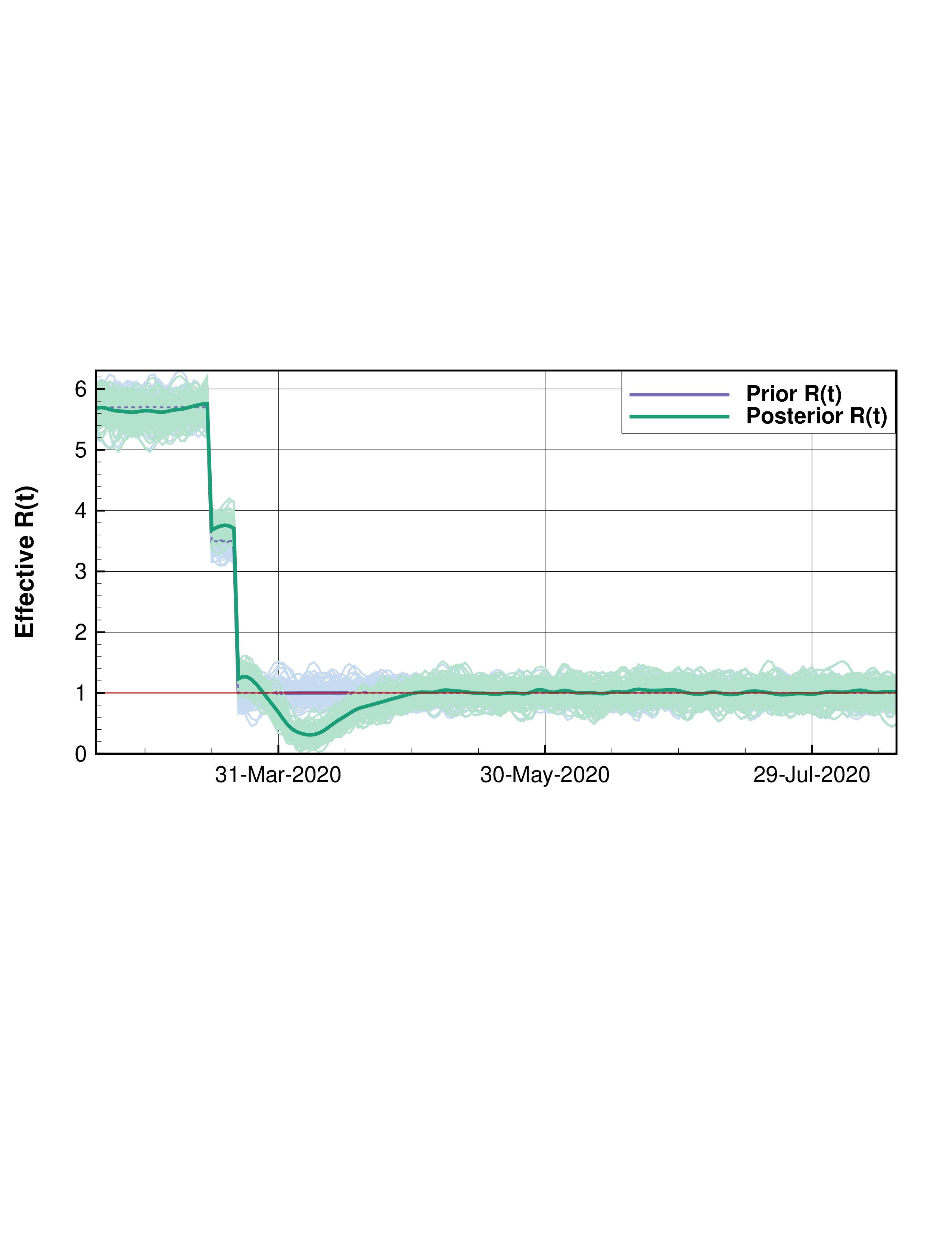
These methods have broad applicability and are only constrained by dimensionallity and the computational cost of the forward model. In addition to the advantage of providing a measure of uncertainty ESMDA can be used to estimate critically important parameters through the combination of the model and available data in the reanalysis sense. A particularly relevant example of recent is the COVID-19 pandemic. In [8] a Susceptible Infected Exposed and Recovered (SEIR) model which was compartmentalized through an age stratified contact rate matrix used ESMDA to estimate important parameters and make short term predictions by a large group of international researchers in their regions. Participating in this effort our group used this model to compare the success of mitigation efforts of four U.S. states by estimating the basic reproduction number of the SARS-CoV-2 virus as a function of time R(t). Shown in Figure  1 is a sample of the results where a gradual step down of R(t) is used starting at dates which correspond to sufficient decreases in mobility data as measured from cell phones. In this figure we highlight that New York achieved a consistent R(t) < 1 implying decreasing cases while California fluctuated around R(t) = 1 during the data window of early March to May 20^th. The model was conditioned on cumulative deaths and daily hospitalizations. Methods like these can be used to preform a reanalysis of the spread of SARS-CoV-2 and tied to other historical data to determine successful strategies and better prepare for the future.

California	New York

The model in [8] has also recently been extended to model sub-populations with transmission between populations possible as well as the provision of a continuous prior on R(t). The sub-populations can represent different countries, states, other localities or population groups with in a locality. In [9] we use cumulative death data reported for different racial/ethnic groups to analyze and study observed disparities in the spread of SARS-CoV-2 across these groups in the United States. We focus on 9 states with the most complete reporting of this data as well as the District of Columbia.

Case: Continuous Updates to R_t(n) (HI)

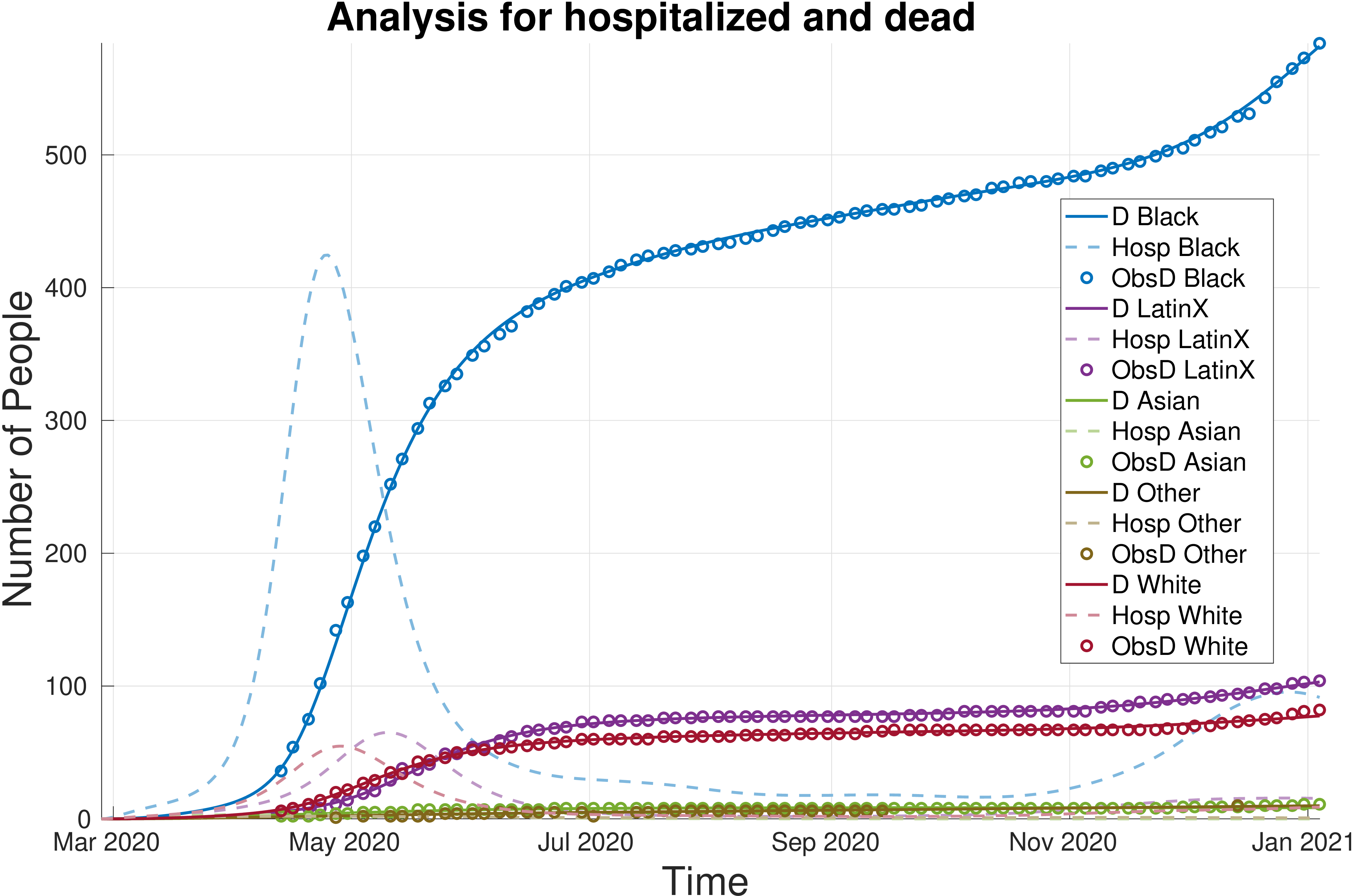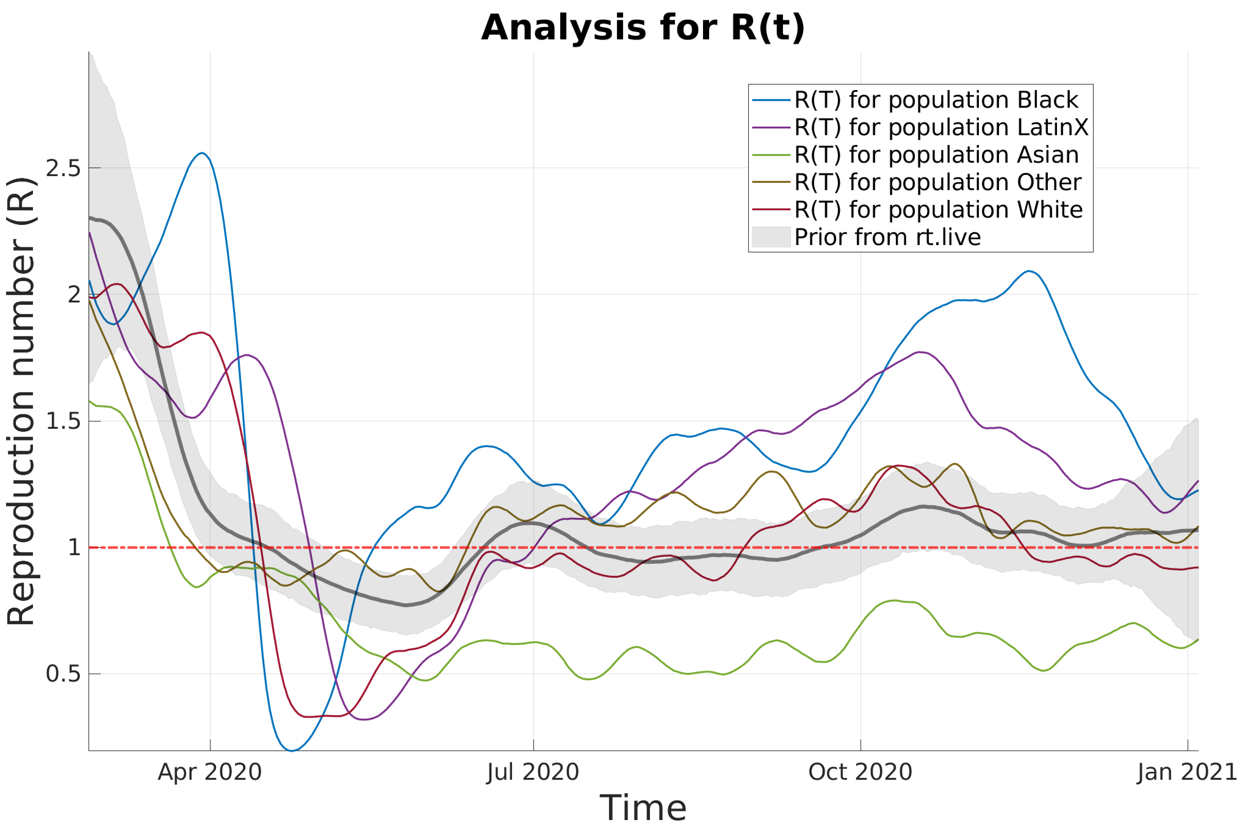In this more recent analysis a continuous prior for the given locality is taken from rt.live and used for all groups and updated based on the death data over time. In Figure  ?? we see the results for the District of Columbia which shows that after the mitigation period (corresponding to the large dip in R(t)) a stratification in the basic reproduction number occurs across the different racial/ethnic groups with the Black and Latinx communities showing the highest rate of spread and more deaths than other groups. This is particularly notable since the Black community is roughly the same proportion of the population of D.C. while the Latinx community only about 11%. We see this as the detection of front-line communities who bores the brunt of the pandemic for a variety of reasons. Methods like ESMDA can be used in this way to shed light on inequity, determine disparity and provide social scientists and policy makers with valuable estimates of critical parameters needed for decision making and equitable actions.

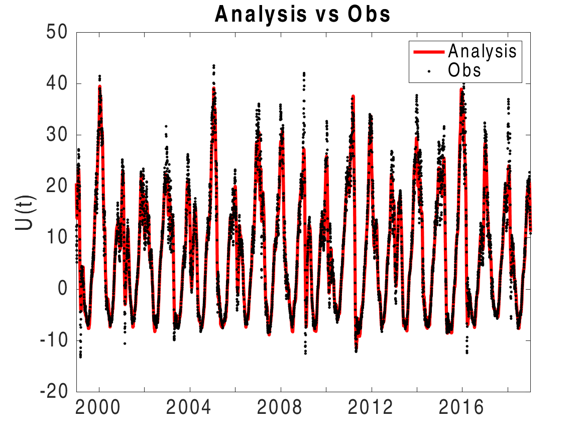
ESMDA was so effective at estimating time dependent parameters related to transmission rates in the previous work we aimed to use it to study a reduced order model of the polar vortex in [34]. In that work we sought to evaluate the representativeness of a reduced order model for the polar vortex originally developed in [28] in the context of the ERA 5 reanalysis data set from ECMWF. We assimilated the reanalysis data to estimate the two main controlling parameters, h (representing perturbations from topography) and λ representing the thermal gradients which drive the polar vortex. We found that when h and λ are allowed to be time dependent we could, through ESMDA parameter estimation, drive the reduced order model in such a way that mean zonal winds represented in the reanalysis data were reproduced. More over the phase space between the mean zonal wind U and parameter λ in this case remained close to the equilibrium solutions of the autonomous version of the system of equations with observe jumping between branches of those solutions. The analysis and phase space are shown in the top row of Figure  3. We then analyzed these recovered time series and found typical signatures of them consistent with their physical meaning around known historical sudden stratospheric warming (SSW) events, bottom row in Figure  3. There we show the same SSW event but with two different decorelation lengths (controlling speed of variation) for the perturbation parameter h. We noted that successful capturing of the data and SSW events was not particularly sensitive to how rapidly h could change. This is somewhat counter intuitive as it is generally understood that perturbations to the vortex from topography cause destabilization of it and one might expect it to be the controlling parameter. However it should be noted that a strong thermal gradient, larger λ, typically leads to a strong polar vortex resistant to perturbations. This suggests perhaps a more subtle interplay between these two parameters highlighted by the ESMDA analysis and pointing to a direction of future research into the interplay between the two.

ESDMA with reduced order model of The Polar Vortex

Future Directions: These methods are widely applicable to a broad range of problems. The ESMDA method is model agnostic at its heart and more complex models than those discussed above could also be employed. This type of data assimilation is also useful for short term forecasting as any number of model parameters can be rapidly estimated providing a following forecast form a now tuned model. I am also interested in studying how climate change has disproportionately affected marginalized groups and see methods like this also useful. Air quality modeling in conjunction with air quality and health data, storm surge and flood models, extreme temperature events and vulnerable populations in conjunction with historical data are just some of the other topics that can be explored. There is also the potential of methods like these to provide undergraduate students with valuable research experience as general codes can be given to them allowing for accessible exploration of a specific model, data assimilation methodology, and relevant data set. The broad application of these methods also provides for broad appeal and can facilitate mentoring opportunities for students from a variety of backgrounds providing an introduction to computational methods along the way. Adding parameter estimation methods like this to a system like JEDI could also enable researchers to explore reduced order models in novel ways.

Ensemble Kalman Filter for Adaptive Moving Mesh Models

Ensemble data assimilation has been widely implemented in weather prediction [18], tumor growth and spread [21], and petroleum reservoir history matching [35]. The ensemble Kalman filter (EnKF) relies on estimates of error statistics using an ensemble of model runs assumed to be Gaussian distributed. The error estimates themselves are calculated using the state vectors (x_i^f) formed from the state variables of each ensemble member. When observations are available each of the N^e ensemble members are updated according to

(3)

Here, y is a vector of observations, h is the operation operator which maps model variables to the observations and K is the Kalman gain matrix and has the form,

(4)

The i^th column of the matrix X^f is formed from the difference between each state vector x_i^f and their mean x^f and normalized by the number of ensemble members minus one. The i^th column matrix Y is formed from the difference between each state vector and mean after applying the observation operator h to each and R^e is the observation error covariance matrix and can also be estimated from the ensemble statistics. The EnKF is often used in a sequential mode by applying updates at times when observations are available and using model to forecast in between.

The EnKF can be directly applied to any forward in time model for which all ensemble members have the same dimension however some adaptations may be needed in special cases such as models which use adaptive mesh solvers. Numerical solvers using adaptive meshes can focus computational power on important regions of a model domain capturing important or unresolved physics. The adaptation can be informed by the model state, external information, or made to depend on the model physics. This has caused AMM schemes to rise in popularity and thus adaptation of DA schemes like the EnKF become important and even advantageous. In recent work we developed an EnKF scheme for a 1-d adaptive mesh solver that in which the nodes are advected with the flow and sometimes deleted if two nodes are too close together (with in a tolerance of δ₁) or inserted if two nodes are two far apart (outside a tolerance of δ₂). While AMM schemes like this are useful to focus computational power in regions of large gradients they present significant challenges for ensemble DA methods. This is because each ensemble member may have a different number of nodes all in different locations making the calculation of the needed error statistics difficult. The different number of nodes can be addressed by interpolating to new nodes for each ensemble member to match the dimension across the ensemble. However, this does not account for the fact that nodes are in different locations and more care is needed. There are two primary options for addressing this, (1) interpolating each ensemble member to the same grid or (2) including the node locations in the state vector paring nodes in some reasonable way. For the scheme described above we use a partitioning of the domain based on the closeness tolerance δ₁. Partitioning the domain into intervals of size δ₁ there is a guarantee that each interval will have at most one point with in it. From there one can map each ensemble member to reference mesh defined by the partition or interpolate new nodes for each ensemble member that does not have a point in a given interval. In the former case the update is done on a regular grid with all nodes in the same location and each ensemble member can be mapped back to the mesh structure it had before the update. In the latter case we include the node locations in the state vector comparing nodes which occupy the same intervals to calculate the needed error statistics for the EnKF. In this way the node locations themselves are updated based on any available physical observations, which are observations of the quantities that drive that flow. While the larger state vector does increase computational cost we did find that the inclusion and update of those node locations improved the assimilation across several metrics including the standard RMSE measure compared to instead only updating the physical quantities on the reference mesh defined by the tolerance δ₁. The models we consider in that work are Burgers equation and the Kuramoto – Sivashinsky equation. In Figure  4 we show the blocks of the error covariance matrices, calculated as X^f(X^f)^T, comparing covariance between the physical values and the node locations themselves. Strikingly we see that the diagonal of that block takes on a very similar shape as that of the first spatial gradient of the solutions highlighting the extra information brought into the update.

Future Directions: While the work described was in 1-d, the complexity and range of patterns that can form in 2-d or 3-d is far greater than is possible in 1-d. This implies that significantly more information may be carried in the cross-covariances between physical values and node locations. Further, if the motivation for the use of an AMM scheme is to focus computational power in regions of strong gradients, updating those node locations in accordance with where observations of those gradients are large may be very advantageous. If the remeshing rules for the AMM model are based on strict considerations of node distances and mesh geometries, a 2-d or 3-d analogue of the reference mesh should be attainable enabling the application of a scheme which includes the mesh in the . An example of such a model is the novel Lagrangian sea ice model neXtSIM [27, 4] which uses a non-conservative adaptive triangular mesh and finite elements. The key to implementing a scheme which updates the mesh is the configuration of an augmented vector that includes variables characterizing the underlying numerical mesh. In 1-d there is little ambiguity as the natural approach is to just add the grid points of the underlying mesh. But in 2-d, the characterization of the “grid” in terms of such vector is not as straightforward when, for instance, using a finite element method. In that case Physical values may be stored at the centers of the elements, where as the elements themselves are determined by their vertices. Considerations of the mesh type, triangular, hexagonal, square etc. also add complications. The development of 2-d or 3-d mesh update schemes is a rich mathematical problem involving numerical analysis, statistics and topology. It also promises to relate to a wide range of applications.

A Hybrid Tangent Linear Model (HTLM) in JEDI

4d-Var is arguably one of the most successful data assimilation techniques in numerical weather prediction in terms of forecast accuracy. Standard strong constraint 4d-Var includes a time series of observations in a costfunction J(x₀) which is minimized for an optimal initial condition x₀ such that the forecast of the model from that initial condition is consistent with the time series of observations in the assimilation window. The future forecast is then run from the end of that window. A critical component of any 4d-Var scheme is the tangent linear model (TLM) and its adjoint, which is essentially the transpose of the TLM. the TLM itself is a linearization of the model in question, which for complex atmospheric models is no small task to implement in code. Many physics parameterizations in these models are complex, full of cases and if statements making ”differentiation” of these schemes difficult. The implement of a TLM is a full time job and when the physics of a model is updated or changed it can require full time employees to update the TLM. Given the success of 4d-Var there is then a desire to find other methods to obtain the TLM with less work, one approach is using ensemble methods to learn it. Learning the entire TLM is computationally intractable, however if we have even an incomplete, perhaps dynamics only, TLM we can use it to our advantage to make it tractable. In this case the TLM advances a model perturbation δx forward in time. When the TLM is incomplete we can refer to it as a simplified tangent linear model (STLM). The HTLM uses an available STLM in conjunction with a nonlinear ensemble to calculate corrective coefficients for the STLM during a 4d-var run [25].

Suppose we have available a simplified TLM M_t−1 (perhaps with incomplete physics) so that

Here the − super script denotes a perturbation advanced by the STLM, a sort of inital guess in perturbation advancement. We will use a non-linear ensemble run and an ensemble of STLM ”first guesses” to find a correction, N₁, which will update δx(t)⁻ at time t₁

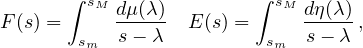
We can find the j^th row of the matrix N₁, v_j, with the equation:

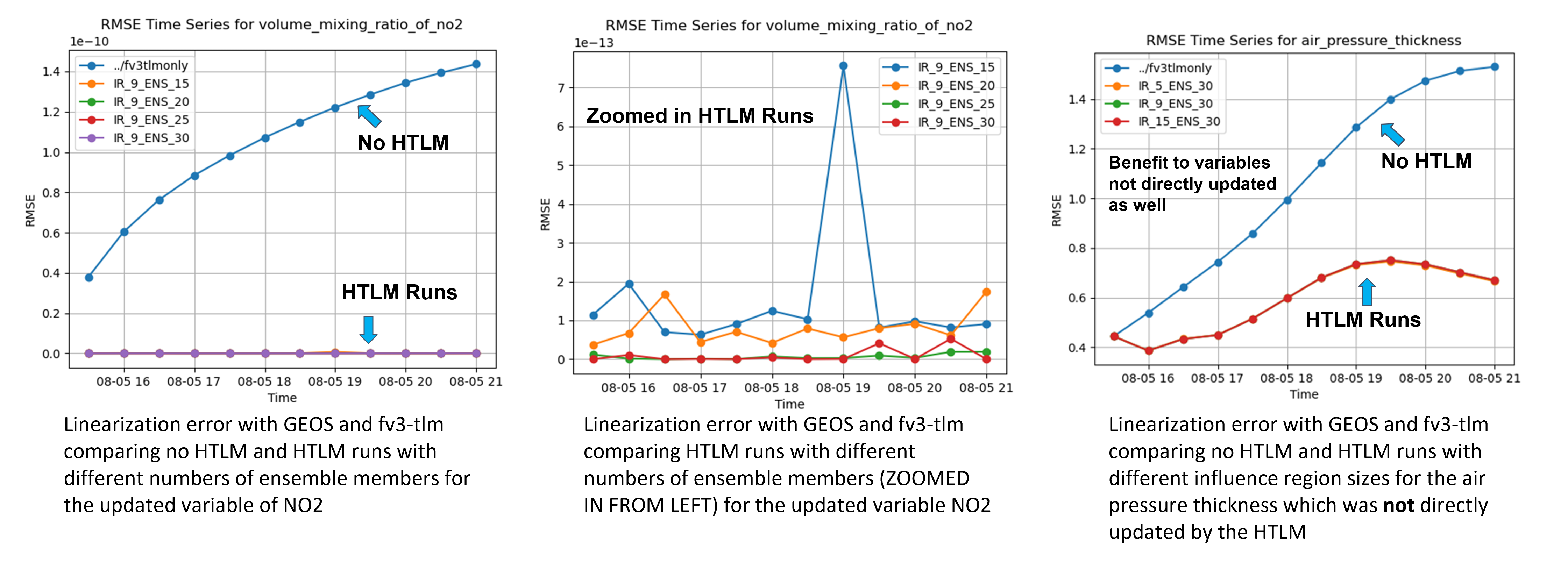
where we have perturbations from the full nonlinear model for the j^th element of the state vector at time t₁ on the right and STLM advanced perturbations sampled around the j^th point with an ”influence region” of size s for each ensemble member. This sets up a set of least squares problems we can then solve for the corrective updates we desire. Once we have said updates we can run 4d -Var normally applying the updates at each subwindow in 4d-var. With the addition of this method to JEDI it is now available for any model with a JEDI interface and is already being tested with NOAA GFS, SOCA, and NASA GEOS with atmospheric chemestry. An example of the reduction in linearization error for NO2 concentrations is shown in Figure  5. This particular method is also intended to be operational at the UK Met Office as a part of their new forecasting system currently underdevelopment.

Future Directions: While the HTLM shows good reduction in linearization error for hight resolutions it can still be computationally intensive and methods to speed things up are desirable. Currently there are already multi-resolution versions of the HTLM available in JEDI but the method could benefit from the ability to calculate and apply update terms on GPU’s. The problem is extremely parallelizable and current work on porting JEDI code to GPU’s is underway. The other expensive piece of this algorithm can be running the nonlinear ensemble, a ML emulator for the nonlinear system would likely be sufficient and allow for larger ensemble sizes, although the HTLM does well with fairly low ensemble numbers already.

New Metrics for Model Calibration

For models which produce coherent structures such as ocean, atmospheric, or sea ice models, comparison of model output to observational data through something like a standard euclidean metric might be misleading or not informative enough. In the presence of coherent structures such as hurricanes, eddies, or sea ice leads one may want to measure model skill with considerations of the geometries as opposed to a simple point by point comparison of values at specific locations. Using the Elastic-Dechohesive rheology the model presented in [38] explicitly represents sea ice leads through discontinuities tracked by a jump vector. While predicting the location of leads is important the shape and orientation of the cracks is also an important consideration and warrants a metric which can take this into account. This can be accomplished by warping the model out put, viewed as an image, to observational data first optimally aligning the leads and then calculating a difference metric. The warping is done with a boundary preserving diffeomorphism and provides two metrics: how close two images can possibly be and how much warping it took to warp one image to another. The space of images considered is the set F = {f : D → Rⁿ|f ∈ C^∞(D)} with dim(D) = m ≤ n they are warped using the set of orientation preserving diffeomorphisims γ ∈ Γ that preserve the boundary of D which forms a group under the operation of composition f ∘ γ. The metric which gives the distance between two images f₁,f₂ ∈ F is defined as,

(5)

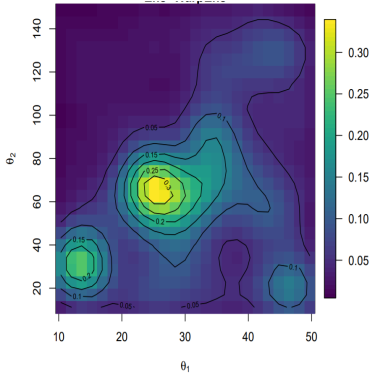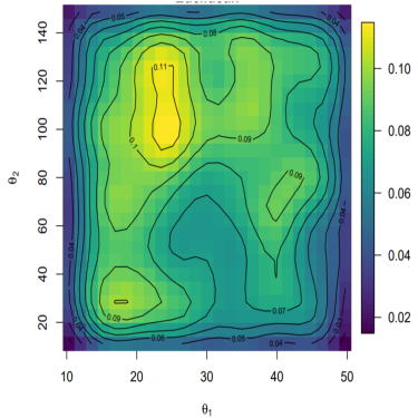This distance, the amplitude distance, satisfies all of the requirements of a proper metric and measures how close two images are after they are optimally aligned by the diffeomorphism γ the amount of warp from this gamma, the phase distance, can also be used as a measure of how different the two images are. These metrics were applied to model out put for the model in [38] compared to SAR satellite imagery for a variety of shear and tensile strength parameters sampled using a latin hyper cube sampling scheme. Using the metrics above a statistical emulator was employed to estimate the optimal parameters based on the data. In Figure  6 we can see that when using the two metrics above a meaningful calibration was obtained while simply using the Euclidean distance provided a flat posterior with little new information. All of the details can be found in [16]

Future Directions: Metrics like these can be applied to a variety of models which produce coherent structures directly. However, finding the optimal gamma is difficult and new optimization techniques, rather than just gradient dissent are desirable. Improving the optimization algorithm is a part of on going work. I also have deep interest in the development of new metrics and studies of which metrics fit a specific situation best. I also am interested in the development of DA methods which assimilate coherent structures based on the geometry in observations as well as the physical values. This could apply to hurricane center locations, ocean currents, sea ice leads, etc.

Machine Learning, Sea Ice and Geophysics

Machine Learning (ML) has become a hot topic in applied mathematics and statistics in recent years owing to the direct utility some of the methods allow. I see ML as powerful for data analysis and an augmentative tool for modeling and forecast. I am currently involved in two projects taking advantage of some of promise of ML techniques to aid in sea ice modeling efforts and as an augmentative tool for Data Assimilation.

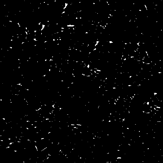
In the first we are exploring the use of a Generative Adversarial Network (GAN) trained on images of melt ponds atop sea ice to generate realistic melt pond geometries and scenes which can serve as input to large scale sea ice models for which parameters may depend on sub-scale processes related to the ponds themselves. For example, ice strength is directly tied to ice thickness in most numerical sea ice models and melt ponds have an effect on the ice thickness over the area which they cover. If, based on thermodynamic variables in the model, the presence of ponds is expected one may wish to generate a statistically consistent melt pond geometry to inform the strength parameter in the ice model. This is particularly important for models wishing to use large ensembles as many realistic melt pond scenes may be needed. Some preliminary results are shown in Figure   7.

GAN Generated	Real Binarized	Area v.s. Perimeter

An additional use for such GAN could be in the aid of sea ice concentration retrievals. In the Arctic summer months melt ponds cover vast areas of sea ice which have the same microwave signature as that of open water. Passive microwave radiometry uses the contrast in microwave signatures of sea ice and open water to estimate sea ice concentration usually at or above the 14km scale. When the melt ponds sit atop the ice they obscure the ice beneath which can cause up to a 30% in sea ice concentration retrieval [20]. If one can rapidly generate sea ice scenes with open water and melt ponds through a well trained GAN, which, are consistent with specific satellite observed microwave radiance. Then it may possible to obtain a measure of uncertainty in what concentrations actually produced the signal. Further, using available validated data it may be possible to train a Deep Neural Net to select the most likely candidate of those possibilities.

The second project looks using ML to replace the observation operator in Data Assimilation. This is motivated by the sea ice concentration example but is a generally applicable idea. The observation operator maps model state variables to the observations space where the predictions and observations may be compared. For passive microwave retrieved sea ice concentrations one may choose to use the concentration value provided by NASA ( with up to 30% due to ponding), for example in which case the observation operator is a simple projection or one may map the sea ice state what would be the observable microwave radiances. The former case is computationally inexpensive and the latter not, especially when using ensemble methods. Assimilating data that may be in in 30% error is undesirable and can be avoided by instead mapping sea ice state to satellite radiance. ML enables this through cuts in computational cost. This concept could apply to many other geophysical systems of interest.

Future Directions: In addition to the projects described above I am also interested in finding ways to use ML to augment models and data assimilation schemes. One of the most obvious places to start is in data processing. The identification of coherent structures or important features such as fronts or sea ice leads would have broad appeal and is an obvious use of ML techniques. There is also the idea of dynamic data thinning, many operational forecasting systems must thin data for assimilation due to computational constraints. A system which identifies important features could choose to increase data resolution there while reducing it in regions of slow dynamics. For models with adaptive meshes, it may also be possible to adapt a system like this to dynamically refocus mesh resolution in areas where more may be needed to capture important dynamics. For computationally expensive models the ability to run large ensembles is often a missing but critical factor in improving forecast skill. This is particularly true with ensemble DA methods where larger ensemble sizes provide better error statistics. While ML can not yet fully replace a numerical model in long term forecasting there has been much progress in providing some short term prediction skill [24, 26]. In the ensemble DA setting this is sufficient as more ensemble members can be created a short time before an observation is available and progressed to the observation time using the ML forecasting scheme. This could potentially allow the use of ensemble methods in cases where computational cost is prohibitive as such. I am also interested in using self learning techniques such a self organizing maps in data analysis in general. ML and its interplay with applied mathematics presents many opportunities.

Wave Dynamics in the Marginal Ice Zone

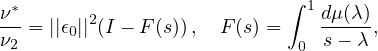
The MIZ can be loosely defined as the region of the ice pack with an ice concentration low enough such that it is significantly effected by ocean swell. Waves propagating into the ice pack play a central role in determining the the break up, distribution, and sizes of ice floes in the MIZ. The ice floes in turn control the dispersion and attenuation of the of the incoming waves. These waves are important to consider in any sea ice model and play a major role in ice melt, shore erosion in the Arctic, and the polar ecosystem. Recently, continuum models have been developed which treat the MIZ as a two-component composite of ice and slushy water [40, 19]. More specifically, the ice-water composite has been modeled as a thin elastic plate, a viscous ice layer atop an inviscid fluid, as well as a viscoelastic layer atop an in-viscid fluid. These models yield dispersion relations which determine the wave properties necessary for continued propagation through the MIZ. At the heart of these models are effective parameters, namely, the effective elasticity, viscosity, and complex viscosity. In practice, these effective parameters, which depend on the composite geometry and the physical properties of the constituents, are quite difficult to measure. To overcome this difficulty, we have employed the tools of homogenization theory to derive bounds on the effective parameters necessary for these models [31]. Specifically, we have developed a Stieltjes integral representation, involving a positive spectral measure of a self-adjoint operator, for the effective complex viscoelasticity ν^∗ of the ice water composite in the low frequency, long wave limit and have the form,

(6)

(7)

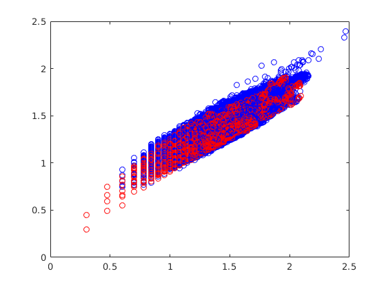
The positivity of the measure allows for the derivation of rigorous forward bounds which depend on partial information about the geometry of the ice-water composite. Integral representations like this have also been used to derive inverse bounds, where measured data is used to bound the structural parameters of the composite, such as the volume factions of the components [5]. We have also developed a simplified wave equation for waves in the ice-water composite. This wave equation arises naturally from the homogenization of the governing equations in the low frequency limit, and could provide a computationally inexpensive numerical model of wave propagation in the MIZ.

General Bounds	Matrix Particle Bounds

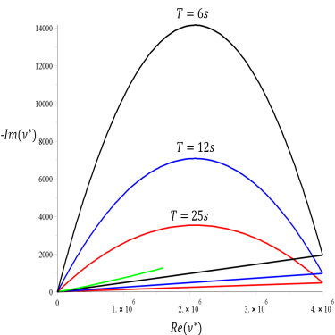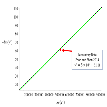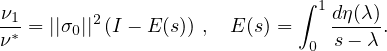
The bounds are shown in Figure  8 as well as an extension of the theory to the matrix-particle bounds valid in pancake ice. Pancake ice consists of small rounded ice floes embedded in a slushy layer typically separated by some small amount. With this particular geometric assumption the support of the measure in the above integral representations may be restricted,

(8)

allowing for a tightening of the original bounds [33, 3]. Here the restriction (s_m,S_M) is governed by the separation of the particles embedded in the matrix. In this case for reasonably chosen individual viscoelasticites of each separate component we obtain much tighter bounds which fall on a data point measured from lab grown pancake ice in a wave tank [41].

Future Directions: Once wave propagation characteristics are understood for a given configuration of ice, the next question is, how does the propagation of the wave affect the configuration? Waves of sufficient amplitude can certainly break up larger ice floes, this changes the geometry and thus the wave propagation characteristics in turn. I am interested in studying this problem through the development of a numerical model of wave propagation and ice break up using some of the results outlined above. The effect that wave propagation has on the floe size and thickness distribution of sea ice is important to consider in any large scale sea ice model. When a floe is broken up by wave action it becomes more susceptible to lateral melting, advection and rafting.

Physical Transport in Sea Ice

Fluid flow through sea ice mediates a broad range of processes such as, snow ice formation, melt pond drainage, and nutrient flux for the algae which call it home. When viewed as a two phase composite of ice and brine pockets, both homogenization theory and percolation theory shed light on the constraining parameter of fluid permeability. Many of the same methods we have applied to fluid flow through sea ice apply to other porous materials such as soil. Beginning with the equations of Stokes flow in the brine pore space and utilizing a two scale expansion, it has been shown that Darcy’s law applies in the limit where the micro structure is much smaller than the composite. Darcy’s law states that the fluid velocity is proportional to the pressure gradient through the effective permeability tensor K^∗. That is, v = −(K^∗∕η)∇P where η is the fluid viscosity. This allows for a direct measurement of the vertical component of K^∗ [10]. The permeability of the ice depends on the connectedness of the brine phase. As the ice warms, the brine pockets begin to form long vertical channels allowing fluid to flow. In columnar ice, the channels first begin to connect on large scales at about ϕ = 5% volume fraction, T = 5^∘C and a bulk salinity of S = 5 parts per thousand, dubbed the rule of fives [13]. Before the critical threshold of ϕ = 5% the ice remains impermeable, while after this threshold the permeability increases rapidly as a function of volume fraction. For granular ice, the critical threshold is significantly higher at about ϕ = 10%, something we experimentally confirmed in Antarctica in 2012 [15]. This behavior can be explained using continuum percolation theory, in particular, we use a compressed powder model [22, 12]. In this model, large polymer spheres of radius R_p are mixed with much smaller metal spheres of radius R_m, and then the mixture is compressed. The main parameter controlling the threshold is the ratio ξ = R_p∕R_m. An approximate formula for the critical volume fraction for percolation of the small metal spheres, when the spheres form long connected chains in the composite, is given by ϕ_c = (1 + ξ𝜃∕(4X_c))⁻¹, where 𝜃 is a reciprocal planar packing factor, and X_c is a critical surface area fraction of the larger particles which must be covered for percolation by the smaller particles [22]. An analysis of the crystalline structure of sea ice yields a model prediction of ϕ ≈ 5% for columnar ice and ϕ ≈ 10% for granular ice [?].

Percolation theory [39, 17, 11] can be used to model transport in disordered materials where the connectedness of one phase, like brine in sea ice, dominates the effective behavior. Consider the square (d = 2) or cubic (d = 3) network of bonds joining nearest neighbor sites on the integer lattice ℤ^d. The bonds are assigned fluid conductivities κ₀ > 0 (open) or 0 (closed) with probabilities p and 1 − p. There is a critical probability p_c, 0 < p_c < 1, called the percolation threshold, where an infinite, connected set of open bonds first appears. In d = 2, p_c = , and in d = 3, p_c ≈ 0.25.

Let κ(p) be the permeability of this random network in the vertical direction. For p < p_c, κ(p) = 0. For p > p_c, near the threshold κ(p) exhibits power law behavior, κ(p) ∼ κ₀(p−p_c)^e as p → p_c⁺, where e is the permeability critical exponent. For lattices, e is believed to be universal, depending only on d, and is equal to t, the lattice electrical conductivity exponent [39, 17, 12, 2]. In d = 3, it is believed [39] that t ≈ 2.0, and there is a rigorous bound [11] that t ≤ 2. Although e can take non-universal values in the continuum, it was shown [39, 17] that for lognormally distributed inclusions, such as those in sea ice, the behavior is universal, with e ≈ 2. The scaling factor k₀ is estimated using critical path analysis [36] and microstructural observations [13]. Thus

with ϕ_c ≈ 0.1 for granular ice and ϕ_c ≈ 0.05 for columnar ice. This model agrees well with measurements in both the Arctic and Antarctic.

References