Lecture 8
Hypothesis Testing Basics
Hypothesis testing is another common form of statistical inference. In hypothesis testing, our objective is to decide whether we have enough evidence to reject the null hypothesis, a statement about the population distribution that a priori we believe to be true, in favor of the alternative hypothesis, a statement about the population disagreeing with the null hypothesis. Usually the null hypothesis is denoted by \(H_0\) and the alternative by \(H_A\).
The first statistical tests introduced to students are tests about the value of a population parameter (other tests are possible, though). These tests generally take the form:
\[H_0: \theta = \theta_o\] \[H_A: \left\{\begin{array}{l} \theta < \theta_0 \\ \theta \neq \theta_0 \\ \theta > \theta_0 \end{array}\right.\]
These are the tests that I discuss.
In statistical testing, one computes a test statistic used to compute a p-value, which represents the probability of observing a test statistic at least as “extreme” as the one actually observed if \(H_0\) were in fact true. Very small p-values indicate a false null hypothesis. Usually what constitutes a “small” p-value is decided beforehand by choosing a level of significance, typically denoted \(\alpha\). If the p-value is less than \(\alpha\), \(H_0\) is rejected in favor of \(H_A\); otherwise, we fail to reject \(H_0\). Common \(\alpha\) include 0.05, 0.01, 0.001, and 0.1. The smaller \(\alpha\), the more difficult it is to reject \(H_0\).
In hypothesis testing, we need to be aware of two types of errors, called Type I and Type II errors. A Type I error is rejecting \(H_0\) when \(H_0\) is true. A Type II error is failing to reject \(H_0\) when \(H_A\) is true. For any test, we want to know the probability of making either type of error. The probability of a Type I error is \(\alpha\), the level of significance; this means we specify beforehand what Type I error we want. Type II errors are much more complicated, since they depend not only on what the true value of \(\theta\) is (which we will call \(\theta_A\), the value of \(\theta\) under the alternative assumed true for Type II error analysis) but additionally on the specified \(\alpha\) and sample size \(n\) (other parameters may be involved as well, but they are assumed constant and unable to be changed). For any testing scheme we represent the Type II error with \(\beta(\theta_A)\), the probability of failing to reject \(H_0\) when the true value of \(\theta\) is \(\theta_A\). Generally \(\beta(\theta_A)\) is large when \(\theta_A\) is close to \(\theta_0\) (in fact, \(\beta(\theta_0) = 1 - \alpha\)), and small when \(\theta_A\) is distant from \(\theta_0\). This should make intuitive sense; a big difference between \(\theta_0\) and \(\theta_A\) should be easy to detect, but a small difference may be more difficult. In practice, researchers pick a \(\theta_A\) for which they want to be able to detect a difference with some specified probability \(\beta\). They then use this to pick a sample size that gives the test the desired property.
Some prefer to discuss the power of a test rather than the probability of a Type II error. The power of a test is the probability of rejecting \(H_0\) when \(\theta = \theta_A\). Power connects both Type I and Type II errors, since the power of a test is defined to be \(\pi(\theta_A) = 1 - \beta(\theta_A)\) and \(\pi(\theta_0) = \alpha\). The same principles discussed with regard to the probability of Type I and Type II errors hold with power.
As with confidence intervals, R has many functions for handling hypothesis testing (in fact, you have already seen most of them). We can perform hypothesis testing “by hand” (not using any functions designed for performing an entire test), or using functions designed for hypothesis testing. We start with methods “by hand”.
Hypothesis Testing “By Hand”
Hypothesis testing “by hand” involves computing the test statistic and finding the appropriate p-value for a test directly. This is the only means of hypothesis testing if a function for performing some desired test does not exist (which is probably not the case unless you’re working with a very obscure test).
Let’s start by considering a simple \(z\)-test, where the hypotheses are:
\[H_0: \mu = \mu_0\] \[H_A: \left\{\begin{array}{l} \mu < \mu_0 \\ \mu \neq \mu_0 \\ \mu > \mu_0 \end{array}\right.\]
The test statistic is \(z = \frac{\bar{x} - \mu_0}{\frac{\sigma}{\sqrt{n}}}\) and the p-value (denoted \(p_{\text{val}}\)) is:
\[p_{\text{val}} = \left\{\begin{array}{lr} \Phi(z) & \text{if } H_A \text{ is } \mu < \mu_0 \\ 2\left(1 - \Phi(|z|)\right) & \text{if } H_A \text{ is } \mu \neq \mu_0 \\ 1 - \Phi(z) & \text{if } H_A \text{ is } \mu > \mu_0 \end{array}\right.\]
This test is unrealistic since it assumes \(\sigma\) is known, but it is simple to analyze.
I demonstrate these procedures by testing whether the diameter of black cherry trees is 12 in. I test the hypotheses:
\[H_0: \mu = 12\] \[H_A: \mu \neq 12\]
I use the data set trees and assume that the population standard deviation is 3. I will base my test on the significance level of \(\alpha = .05\).
# Some basic numbers
xbar <- mean(trees$Girth)
xbar
## [1] 13.24839n <- nrow(trees)
mu_0 <- 12
sigma <- 3
# Test statistic
z <- (xbar - mu_0)/(sigma/sqrt(n))
z## [1] 2.316908# Get p-value, using pnorm
pval <- 2 * (1 - pnorm(abs(z)))
pval## [1] 0.02050872Since 0.02 is less than my significance level of .05, I reject the null hypothesis; the mean diameter of black cherry trees is not 12. That said, if I were to use a significance level of \(\alpha = .01\), I would not reject the null hypothesis. Remember that the p-value represents the largest level of significance at which I would fail to reject the null hypothesis. Thus the p-value measures how unlikely my data is if the null hypothesis were true, with smaller p-values indicating more evidence against the null hypothesis.
Testing hypotheses “by hand” follows a similar format to the one demonstrated here, so I do not demonstrate this approach any more in this lecture.
R Functions for Statistical Testing
R has functions for performing many common statistical tests, including many that come with any R installation in the stats package. We already saw all the functions for performing statistical tests I consider in this lecture when we discussed confidence intervals. There may be additional parameters to specify depending on the statistical test, such as what the population mean under the null hypothesis is, but otherwise little has changed. Many of these functions have a common parameter alternative that determines what the alternative hypothesis is. For a two-sided test (that is, when the alternative hypothesis is that \(\theta \neq \theta_0\)), you may set alternative = "two.sided" (this is the default, though, so setting this may not be necessary). If the alternative hypothesis says \(\theta > \theta_0\), set alternative = "greater", and if the alternative hypothesis says \(\theta < \theta_0\), set alternative = "less".
The statistical testing functions in stats will report the results of a statistical test and many other important quantities, such as the estimate of the parameters investigated, the sample size, degrees of freedom, the value of a test statistic, the p-value, and even the corresponding confidence interval. They do not state whether to reject or not reject the null hypothesis; you are expected to tell from the p-value reported whether to reject or not reject based on the significance level you have chosen.
stats includes some functions for Type II error analysis (often in the form of power analysis, which amounts to the same sort of analysis), but this is a difficult analysis in general. Functions for study planning may be included in other packages.
Test for Location of Population Mean
Suppose you wish to test the hypotheses:
\[H_0: \mu = \mu_0\] \[H_A: \left\{\begin{array}{l} \mu < \mu_0 \\ \mu \neq \mu_0 \\ \mu > \mu_0 \end{array}\right.\]
Furthermore, you assume (after perhaps using qqnorm() or some other procedure to check) that your data is Normally distributed, and thus it is safe to use the \(t\)-test (or your sample size is large enough for this to be safe to use anyway). The function t.test() allows you to test these hypotheses. The call t.test(x, mu = mu0) will test whether the data stored in vector x has a mean of mu0 or whether the true mean differs from mu0 (remember: change the form of the alternative hypothesis with the parameter alternative), using the test statistic:
\[t = \frac{\bar{x} - \mu_0}{\frac{s}{\sqrt{n}}}\]
I test the hypotheses regarding tree girth in the trees data set mentioned earlier in this lecture, but this time using t.test(), using a level of significance of \(\alpha = .05\).
# Check the normality assumption
qqnorm(trees$Girth)
qqline(trees$Girth)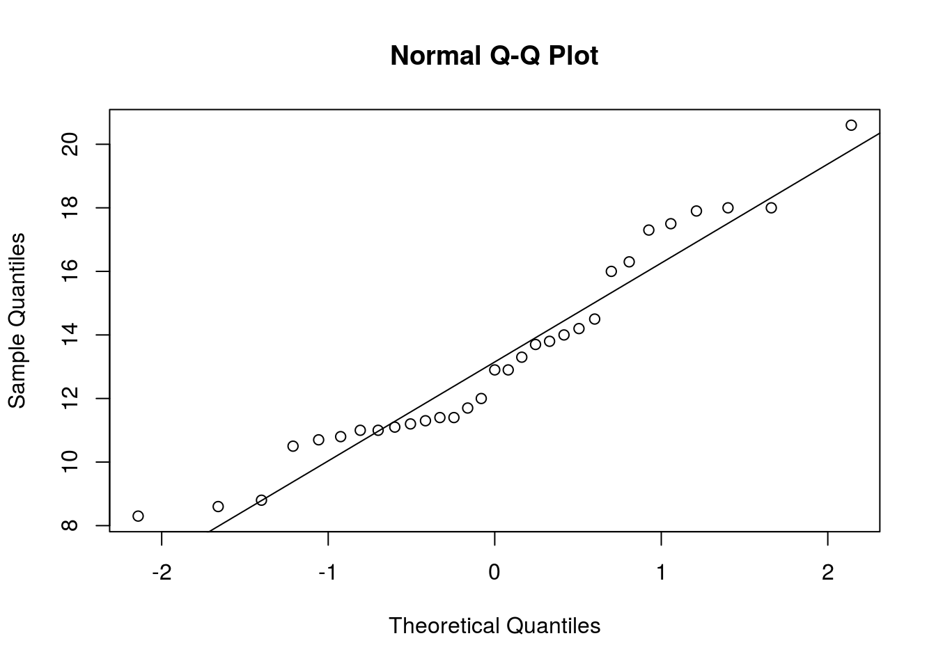
# Data appears Normally distributed, so it's safe to use t.test
t.test(trees$Girth, mu = 12)
##
## One Sample t-test
##
## data: trees$Girth
## t = 2.2149, df = 30, p-value = 0.0345
## alternative hypothesis: true mean is not equal to 12
## 95 percent confidence interval:
## 12.09731 14.39947
## sample estimates:
## mean of x
## 13.24839With a p-value of 0.0345, I reject the null hypothesis in favor of the alternative.
Test for Value of a Proportion
Suppose you wish to test the hypotheses:
\[H_0: p = p_0\] \[H_A: \left\{\begin{array}{l} p < p_0 \\ p \neq p_0 \\ p > p_0 \end{array}\right.\]
Suppose your sample size is large enough to invoke the Central Limit Theorem to describe the sampling distribution of the statistic \(\hat{p} = \frac{1}{n}\sum_{i = 1}^{n} X_i\), and thus use the test statistic:
\[z = \frac{\hat{p} - p_0}{\sqrt{\frac{p_0(1 - p_0)}{n}}}\]
You can use prop.test() to test the hypotheses if these conditions hold. The call prop.test(x, n, p = p0) will test whether the true proportion is p0 when there were x successes out of n trials (both x and n are single non-negative integers).
Suppose that out of 1118 survey participants, 562 favored Hillary Clinton over Donald Trump (this data is fictitious). I test whether the candidates are tied or whether Hillary Clinton is winning below:
prop.test(562, 1118, alternative = "greater", p = 0.5)##
## 1-sample proportions test with continuity correction
##
## data: 562 out of 1118, null probability 0.5
## X-squared = 0.022361, df = 1, p-value = 0.4406
## alternative hypothesis: true p is greater than 0.5
## 95 percent confidence interval:
## 0.477664 1.000000
## sample estimates:
## p
## 0.5026834With a p-value of 0.4406, I soundly fail to reject the null hypothesis.
Suppose that your sample size is not large enough to use the above procedure (or you would simply rather not risk it), and you would rather use the binomial distribution to perform an exact test of the null and alternative hypotheses. binom.test() will allow you to perform such a test with a function call similar to prop.test().
Suppose you wish to know what the political alignment of your Facebook friends are. You conduct a survey, randomly selecting 15 friends from your friends list and determining their political affiliation, with a “success” being a friend being the same political party as yours. You find that 10 of your friends have the same political views as you, and use this to test whether most of your friends agree with you. You use a significance level of \(\alpha = .1\) to decide whether to reject the null hypothesis.
binom.test(10, 15, p = .5, alternative = "greater")##
## Exact binomial test
##
## data: 10 and 15
## number of successes = 10, number of trials = 15, p-value = 0.1509
## alternative hypothesis: true probability of success is greater than 0.5
## 95 percent confidence interval:
## 0.4225563 1.0000000
## sample estimates:
## probability of success
## 0.6666667Since the p-value of 0.1509 is greater than the significance level, you fail to reject the null hypothesis.
Testing for Difference Between Population Means Using Paired Data
Suppose you have data sets from two populations \(X_i\) and \(Y_i\), each possibly having their own mean, and you wish to test:
\[H_0: \mu_X = \mu_Y \equiv \mu_X - \mu_Y = 0\] \[H_A: \left\{\begin{array}{l} \mu_X < \mu_Y \equiv \mu_X - \mu_Y < 0 \\ \mu_X \neq \mu_Y \equiv \mu_X - \mu_Y \neq 0 \\ \mu_X > \mu_Y \equiv \mu_X - \mu_Y > 0 \end{array}\right.\]
Since the data is paired, testing these hypotheses is similar to inference with univariate data after you find \(D_i = X_i - Y_i\) and replace \(\mu_X - \mu_Y\) with \(\mu_D\).
If the differences \(D_i\) are Normally distributed, you can use the \(t\)-test to decide whether to reject \(H_0\) (you would also use the \(t\)-test if your data was not Normally distributed but the sample size was large enough that little would change if a more exact test were used). In R, use t.test() setting the parameter paired = TRUE. By default the parameter mu is 0, so you do not need to change it unless you want to test for a difference between the two populations other than zero. (In other words, you would be testing whether the samples differ by a certain amount as opposed to whether they differ at all.)
Below I test whether stronger speed limits reduce accidents, using the Swedish study we saw in the lecture on confidence intervals (in fact, you may see that most of the following code is identical to that lecture’s code). I will reject \(H_0\) if the p-value is less than 0.1.
library(MASS)
library(reshape)
head(Traffic)
## year day limit y
## 1 1961 1 no 9
## 2 1961 2 no 11
## 3 1961 3 no 9
## 4 1961 4 no 20
## 5 1961 5 no 31
## 6 1961 6 no 26# The Traffic data set needs to be formed into a format that is more easily worked with. The following code reshapes the data into a form that allows for easier comparison of paired days
new_Traffic <- with(Traffic, data.frame("year" = year, "day" = day, "limit" = as.character(limit), "y" = as.character(y)))
melt_Traffic <- melt(new_Traffic, id.vars = c("year", "day"), measure.vars = c("limit", "y"))
form_Traffic <- cast(melt_Traffic, day ~ year + variable)
form_Traffic <- with(form_Traffic, data.frame("day" = day, "limit_61" = `1961_limit`, "accidents_61" = as.numeric(as.character(`1961_y`)), "limit_62" = `1962_limit`, "accidents_62" = as.numeric(as.character(`1962_y`))))
head(form_Traffic)## day limit_61 accidents_61 limit_62 accidents_62
## 1 1 no 9 no 9
## 2 2 no 11 no 20
## 3 3 no 9 no 15
## 4 4 no 20 no 14
## 5 5 no 31 no 30
## 6 6 no 26 no 23# Now we subset this data so that only days where speed limits were enforced differently between the two years
diff_Traffic <- subset(form_Traffic, select = c("accidents_61", "accidents_62", "limit_61", "limit_62"), subset = limit_61 != limit_62)
head(diff_Traffic)## accidents_61 accidents_62 limit_61 limit_62
## 11 29 17 no yes
## 12 40 23 no yes
## 13 28 16 no yes
## 14 17 20 no yes
## 15 15 13 no yes
## 16 21 13 no yes# Get a vector for accidents when the speed limit was not enforced, and a vector for accidents for when it was
accident_no_limit <- with(diff_Traffic, c(accidents_61[limit_61 == "no"], accidents_62[limit_62 == "no"]))
accident_limit <- with(diff_Traffic, c(accidents_61[limit_61 == "yes"], accidents_62[limit_62 == "yes"]))
accident_limit## [1] 19 19 9 21 22 23 14 19 15 13 22 42 29 21 12 16 17 23 16 20 13 13 9
## [24] 10 27 12 7 11 15 29 17 17 15 25 9 16 25 25 16 22 21 17 26 41 25 12
## [47] 17 24 26 16 15 12 22 24 16 25 14 15 9accident_no_limit## [1] 29 40 28 17 15 21 24 15 32 22 24 11 27 37 32 25 20 40 21 18 35 21 25
## [24] 34 42 27 34 47 36 15 26 21 39 39 21 15 17 20 24 30 25 8 21 10 14 18
## [47] 26 38 31 12 8 22 17 31 49 23 14 25 24# It took a lot of work, but finally we have the data in a format we want. Now, the first thing I check is whether the differences are Normally distributed
qqnorm(accident_limit - accident_no_limit)
qqline(accident_limit - accident_no_limit)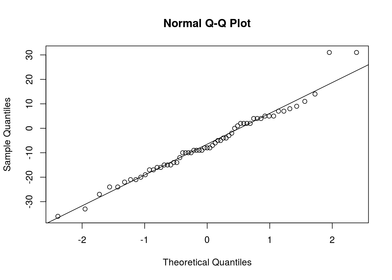
# Aside from a couple observations, the Normal distribution seems to fit very well. t procedures are safe to use.
t.test(accident_limit, accident_no_limit, paired = TRUE, alternative = "less")
##
## Paired t-test
##
## data: accident_limit and accident_no_limit
## t = -3.7744, df = 58, p-value = 0.0001897
## alternative hypothesis: true difference in means is less than 0
## 95 percent confidence interval:
## -Inf -3.588289
## sample estimates:
## mean of the differences
## -6.440678With a p-value of 0.0002, we soundly reject \(H_0\).
Test for Difference in Mean Between Populations With Independent Samples
Again, consider the set of hypotheses considered in the above section, only the data is not paired; we have two samples, \(X_1, ..., X_n\) and \(Y_1, ..., Y_m\) (I assume both are drawn from Normal distributions, so we may use \(t\) procedures). Our test statistic depends on whether we believe our populations are homoskedastic (common standard deviation \(\sigma\)) or heteroskedastic (possibly differing standard deviations \(\sigma_X\) and \(\sigma_Y\)) under the null hypothesis (whether they are homoskedastic or heteroskedastic if the alternative hypothesis is true doesn’t matter). If we believe that, under \(H_0\), the populations are homoskedastic, our test statistic will be:
\[t = \frac{\bar{x} - \bar{y}}{s\sqrt{\frac{1}{n} + \frac{1}{m}}}\]
where \(s\) is the pooled sample standard deviation. The degrees of freedom of the \(t\) distribution used to compute the p-value are \(\nu = n + m - 2\).
If we do not assume that the populations are homoskedastic under \(H_0\) (so we either believe they are heteroskedastic or that we have no reason to believe they are homoskedastic and thus assume heteroskedasticity by default), our test statistic will be:
\[t = \frac{\bar{x} - \bar{y}}{\sqrt{\frac{s_x^2}{n} + \frac{s_y^2}{m}}}\]
The \(t\) distribution is used as an approximation of the true distribution this test statistic follows under \(H_0\), with degrees of freedom:
\[\nu = \frac{\left(\frac{s_X^2}{n} + \frac{s_Y^2}{m}\right)^2}{\frac{\left(s_X^2/n\right)^2}{n - 1} + \frac{\left(s_Y^2/m\right)^2}{m - 1}}\]
t.test() allows for testing these hypotheses. There is no need to set paired = FALSE, and you only set var.equal = TRUE if you want a test assuming that the populations are homoskedastic under \(H_0\). (If this assumption holds, the homoskedastic test is more powerful than the heteroskedastic test, but the difference is only minor.)
Let’s test whether orange juice increases the tooth growth of guinea pigs, using the ToothGrowth data set. I use a significance level of \(\alpha = .05\) to decide whether to reject \(H_0\).
# First, let's get the data into separate vectors
split_len <- split(ToothGrowth$len, ToothGrowth$supp)
OJ <- split_len$OJ
VC <- split_len$VC
# Perform statistical test
t.test(OJ, VC, alternative = "greater")
##
## Welch Two Sample t-test
##
## data: OJ and VC
## t = 1.9153, df = 55.309, p-value = 0.03032
## alternative hypothesis: true difference in means is greater than 0
## 95 percent confidence interval:
## 0.4682687 Inf
## sample estimates:
## mean of x mean of y
## 20.66333 16.96333# Is there homoskedasticity? Let's check a boxplot
boxplot(len ~ supp, data = ToothGrowth)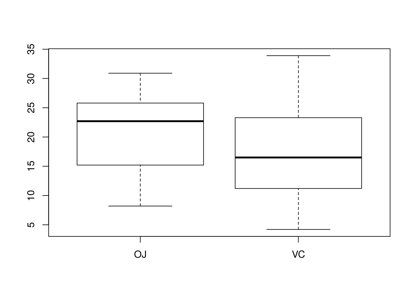
# These populations look homoskedastic; spread does not differ drastically
# between the two. A test that assumes homoskedasticity is thus performed.
t.test(OJ, VC, var.equal = TRUE, alternative = "greater")
##
## Two Sample t-test
##
## data: OJ and VC
## t = 1.9153, df = 58, p-value = 0.0302
## alternative hypothesis: true difference in means is greater than 0
## 95 percent confidence interval:
## 0.4708204 Inf
## sample estimates:
## mean of x mean of y
## 20.66333 16.96333# Not much changed.In both versions of the test, I reject the null hypothesis.
Testing for Difference in Population Proportion
Suppose you have two data sets of Bernoulli random variables, \(X_1, ..., X_n\) and \(Y_1, ..., Y_m\), and you wish to know if the population proportion of “successes” for the first population, \(p_X\), differs from the corresponding proportion in the second population, \(p_Y\). Your set of hypotheses are:
\[H_0: p_X = p_Y \equiv p_X - p_Y = 0\] \[H_A: \left\{\begin{array}{l} p_X < p_Y \equiv p_X - p_Y < 0 \\ p_X \neq p_Y \equiv p_X - p_Y \neq 0 \\ p_X > p_Y \equiv p_X - p_Y > 0 \end{array}\right.\]
If \(m\) and \(n\) are reasonably large, the Central Limit Theorem can be used to obtain a test statistic:
\[z = \frac{\hat{p}_X - \hat{p}_Y}{\sqrt{\hat{p}(1 - \hat{p})\left(\frac{1}{n} + \frac{1}{m} \right)}}\]
where \(\hat{p}\) is the pooled sample proportion (that is, the proportion of “successes” from the combined sample). Under \(H_0\), this test statistic follows a standard Normal distribution (when applying the Central Limit Theorem).
In R, prop.test() can be used to conduct this test, using a call similar to prop.test(x, n) where x is a vector containing the number of successes in the samples, and n is the size of both samples.
Below, I use prop.test() and the Melanoma data set to test whether males and females are equally likely to die from melanoma after being diagnosed, or whether they differ. I use a significance level of \(\alpha = .05\).
# First, I obtain sample sizes, using the fact that sex == 1 for males and 0
# for females
n <- c(Female = nrow(Melanoma) - sum(Melanoma$sex), Male = sum(Melanoma$sex))
# Now, find how many in each group died from melanoma
x <- aggregate(Melanoma$status == 1, list(Melanoma$sex), sum)
x <- c(Female = x[1, "x"], Male = x[2, "x"])
prop.test(x, n)
##
## 2-sample test for equality of proportions with continuity
## correction
##
## data: x out of n
## X-squared = 4.3803, df = 1, p-value = 0.03636
## alternative hypothesis: two.sided
## 95 percent confidence interval:
## -0.283876633 -0.005856138
## sample estimates:
## prop 1 prop 2
## 0.2222222 0.3670886With a p-value of 0.0364, I reject the null hypothesis; men and women are not equally likely to die from melanoma.
Power Analysis
Power analysis is an important part of planning a statistical study. Researchers usually try to make a test as powerful as reasonable (there is always a more powerful study than the one currently employed; simply use a sample size of \(n + 1\) rather than \(n\)). A useful technique in planning a study is to decide what effect size the test should be able to detect with some specified probability, then choose a sample size that will give this property to the test.
Whole R packages are devoted to providing tools for study planning, but the stats package included with any R installation has some function for power analysis, including those for the two classes of tests we have studied: tests for population mean, and tests for population proportion.
Power Analysis for the \(t\)-Test
power.t.test() allows you to perform power analysis for the \(t\)-test. It can be used in different ways depending on which parameters are passed to it and which are set to NULL, and you are encouraged to read the documentation (with, say, help("power.t.test")) to see how this function behaves, but I will focus on two applications: computing power for a test, and computing a sample size for a given power.
power.t.test(n, delta, sd, sig.level, type = "some.type.of.test", alternative = "some.alternative") will compute the power of a test with sample size n, where the difference between the mean under the null hypothesis and the mean under the alternative hypothesis, \(\mu_0 - \mu_A\), is delta, the population standard deviation is sd, and the significance level is sig.level (by default, sig.level = .05). The type of the test administered is specified by type, and can be either "one.sample", "two.sample", or "paired" (the meaning should be self-evident). alternative specifies whether the alternative hypothesis is one-sided or two-sided. Notice that if alternative = "two.sided", delta will be perceived as also communicating which direction the difference between \(\mu_0\) and \(\mu_A\) occurs, so if you want the power to include the probability of rejecting in the opposite direction as well, you should set the parameter strict to TRUE (by default, strict = FALSE).
Suppose you plan to conduct a study to determine whether a new drug would induce weight loss. You plan to give all study participants both the drug and a placebo (in random order, with neither the study participants or experiment staff knowing which treatment is the drug or placebo, thus helping combat bias), and measure the difference in weight loss when the two treatments are administered. Thus your hypotheses are:
\[H_0: \mu_{\text{drug}} = \mu_{\text{placebo}}\] \[H_A: \mu_{\text{drug}} > \mu_{\text{placebo}}\]
Your test will use a significance level of \(\alpha = .01\). You believe that \(\sigma = 20\) (you estimate high to be on the safe side). A researcher on staff suggests a sample size of 20. You are skeptical that a study with that sample size will be able to detect a five-pound difference in weight loss between the drug and the placebo, and thus compute \(\pi(5)\), the power of the test when the true difference is 5 lbs.
power.t.test(n = 20, delta = 5, sd = 20, sig.level = 0.01, type = "paired",
    alternative = "one.sided")
##
## Paired t test power calculation
##
## n = 20
## delta = 5
## sd = 20
## sig.level = 0.01
## power = 0.09924502
## alternative = one.sided
##
## NOTE: n is number of *pairs*, sd is std.dev. of *differences* within pairsThis study will only detect a five-pound difference about 10% of the time, which is too low for your liking. You want to find a sample size to guarantee detecting this difference with some higher probability. This may involve a much larger sample size.
power.t.test(delta = d, sd = s, sig.level = alpha, power = p, type = "some.type.of.test", alternative = "some.alternative") is similar in usage to the earlier command but instead of finding power, the sample size will be found such that the power of the test when the difference between \(\mu_0\) and \(\mu_A\) is d is power. Thus this call is useful when planning a test and choosing an appropriate sample size for detecting a specified effect with some desired probability.
You have decided that you want the study to detect a five-pound difference in weight loss 90% of the time, and want to find a sample size that will give your test this property. You use R to find this sample size:
power.t.test(power = 0.9, delta = 5, sd = 20, sig.level = 0.01, type = "paired",
    alternative = "one.sided")
##
## Paired t test power calculation
##
## n = 210.9878
## delta = 5
## sd = 20
## sig.level = 0.01
## power = 0.9
## alternative = one.sided
##
## NOTE: n is number of *pairs*, sd is std.dev. of *differences* within pairsThe results suggest that you need 211 study participants for your study to have the desired property.
Power Analysis for Tests of Proportion
power.prop.test() does for tests for population proportion what power.t.test() does for tests for population mean. The syntax is similar, except there is no parameter type, and delta is replaced with p1 and p2, which specify the population proportions under the two hypotheses. (There is no need to specify sd, so clearly that is not a parameter either.)
Gallup polls often survey samples of 1500 adults. Suppose a Gallup poll asks individuals whether they support Hillary Clinton or Donald Trump for President, and the poll uses a significance level of \(\alpha = .05\) (the default for power.prop.test(), thus allowing us to ignore the parameter sig.level). Suppose we wish to use the results of the poll to test:
\[H_0: p = .5\] \[H_A: p > .5\]
where \(p\) is the proportion of the population supporting Hillary Clinton. We would like to know if the Gallup poll can reasonably detect a 1% advantage for Clinton, and use power.prop.test() to detect this:
power.prop.test(n = 1500, p1 = .5, p2 = .51, alternative = "one.sided")##
## Two-sample comparison of proportions power calculation
##
## n = 1500
## p1 = 0.5
## p2 = 0.51
## sig.level = 0.05
## power = 0.136286
## alternative = one.sided
##
## NOTE: n is number in *each* groupThe Gallup poll will detect this difference only 14% of the time. If we wanted to detect this advantage for Clinton 95% of the time, what sample size do we need? By specifying power = .95 and omitting n, we can find the desired sample size.
power.prop.test(power = .95, p1 = .5, p2 = .51, alternative = "one.sided")##
## Two-sample comparison of proportions power calculation
##
## n = 54102.75
## p1 = 0.5
## p2 = 0.51
## sig.level = 0.05
## power = 0.95
## alternative = one.sided
##
## NOTE: n is number in *each* groupWe would need a sample size of 54,103 people to have a test with these properties.
p-Hacking
p-hacking (also known as data dredging or other names) is the practice of reformulating hypotheses and research questions and computing p-values for the same data set until a statistically significant result is obtained. This is considered to be very bad practice, and results found by p-hacking are untrustworthy. The probability of a Type I error is inflated when p-hacking is used, yet nowhere is this communicated or adjusted for. You do not want to be accused of p-hacking.
When conducting a study, you should have a well-defined problem prior to any testing. Exploratory analysis with visualization, or deeper analysis on small subsets of the data (that you do not use later when testing) You should also report what you did. If you perform an analysis and do not get the results you expected and you are certain that the analysis was done correctly, or you simply are unsatisfied with the conclusion, you need to perform analysis on new data, not the same data. Furthermore, you should report any prior analyses. Keep in mind that if you perform lots of tests and end when you find a significant result, you may be p-hacking, especially if you do not report that this was done.
There are many do’s and don’t’s with regards to how to properly conduct hypothesis testing and avoid p-hacking. Some rules of thumb would be to have a well-defined plan and research question prior to analysis and keep statistical testing critical to the research question at a minimum. The website FiveThirtyEight has made a web app where you can see what p-hacking is and why it cannot be trusted.