Lecture 7
Confidence Interval Basics
The sample mean, \(\bar{x}\), is usually not considered enough to know where the true mean of a population is. It is seen as one instantiation of the random variable \(\overline{X}\), and since we interpret it as being the result of a random process, we would like to describe the uncertainty we associate with its position relative to the population mean. This is true not only of the sample mean but any statistic we estimate from a random sample.
The last lecture was concerned with computational methods for performing statistical inference. In this lecture, we consider procedures for inferential statistics derived from probability models. In particular, I focus on parametric methods, which aim to uncover information regarding the location of a parameter of a probability model assumed to describe the data, such as the mean \(\mu\) in the Normal distribution, or the population proportion \(p\). (The methods explored last lecture, such as bootstrapping, are non-parametric; they do not assume a probability model describing the underlying distribution of the data. MATH 3080 covers other non-parametric methods.)
Why use probabilistic methods when we could use computational methods for many procedures? First, computational power and complexity may limit the effectiveness of computational methods; large or complex data sets may be time consuming to process using computational methods alone. Second, methods relying on simulation, such as bootstrapping, are imprecise. Many times this is fine, but the price of imprecision is large when handling small-probability events and other contexts where precision is called for. Third, while computational methods are robust (deviation from underlying assumptions has little effect on the end result), this robustness comes at the price of power (the ability to detect effects, even very small ones), and this may not be acceptable to a practitioner (much of statistical methodology can be seen as a battle between power and robustness, which are often mutually exclusive properties). Furthermore, many computational methods can be seen as a means to approximate some probabilistic method that is for some reason inaccessible or not quite optimal.
A \(100C\)% confidence interval is an interval or region constructed in such a way that the probability the procedure used to construct the interval results in an interval containing the true population parameter of interest is \(C\). (Note that this is not the same as the probability that the parameter of interest is in the confidence interval, which does not even make sense in this context since the confidence interval computed from the sample is fixed and the parameter of interest is also considered fixed, albeit unknown; this is a common misinterpretation of the meaning of a confidence interval and I do not intend to spread it.) We call \(C\) the confidence level of the confidence interval. Smaller \(C\) result in intervals that capture the true parameter less frequently, while larger \(C\) result in intervals capturing the desired parameter more frequently. There is (always) a price, though; smaller \(C\) yield intervals that are more precise (and more likely to be wrong), while larger \(C\) yield intervals that are less precise (and less likely to be wrong). There is usually only one way to get more precise confidence intervals while maintaining the same confidence level \(C\): collect more data.
In this lecture we consider only confidence intervals for univariate data (or data that could be univariate). When discussing confidence intervals, the estimate is the estimated value of the parameter of interest, and the margin of error (which I abbreviate with “moe”) is the quantity used to describe the uncertainty associated with the estimate. The most common and familiar type of confidence interval is a two-sided confidence interval of the form:
\[\text{estimate} \pm \text{moe}\]
For estimates of parameters from symmetric distributions, such a confidence interval is called an equal-tail confidence interval (so called because the confidence interval is equally likely to err on either side of the estimate). For estimates for parameters from non-symmetric distributions, an equal-tail confidence interval may not be symmetric around the estimate. Also, confidence intervals need not be two-sided; one-sided confidence intervals, which effectively are a lower-bound or upper-bound for the location of the parameter of interest, may also be constructed.
Confidence Intervals “By Hand”
One approach for constructing confidence intervals in R is “by hand”, where the user computes the estimate and the moe. This approach is the only one available if no function for constructing the desired confidence interval exists (that will not be the case for the confidence intervals we will see, but may be the case for others).
Let’s consider a confidence interval for the population mean when the population standard deviation is known. The estimate is the sample mean, \(\bar{x}\), and the moe is \(z_{\frac{1 - C}{2}}\frac{\sigma}{\sqrt{n}}\), where \(C\) is the confidence level, \(z_{\alpha}\) is the quantile of the standard Normal distribution such that \(P(Z > z_{\alpha}) = 1 - \Phi(z_{\alpha}) = \alpha\), \(\sigma\) is the population standard deviation (presumed known, which is unrealistic), and \(n\) is the sample size. So the two-sided confidence interval is:
\[\bar{x} \pm z_{\frac{1 - C}{2}}\frac{\sigma}{\sqrt{n}}\]
Such an interval relies on the Central Limit Theorem to ensure the quality of the interval. For large \(n\), it should be safe (with “large” meaning over 30, according to DeVore), and otherwise one may want to look at the shape of the distribution of the data to decide whether it is safe to use these procedures (the more “Normal”, the better).
The “by hand” approach finds all involved quantities individually and uses them to construct the confidence intervals.
Let’s construct a confidence interval for sepal length of versicolor iris flowers in the iris data set. There are 50 observations, so it should be safe to use the formula for the CI described above. We will construct a 95% confidence interval assume that \(\sigma = 0.5\).
# Get the data
vers <- split(iris$Sepal.Length, iris$Species)$versicolor
xbar <- mean(vers)
xbar
## [1] 5.936# Get critical value for confidence level
zstar <- qnorm(0.025, lower.tail = FALSE)
sigma <- 0.5
# Compute margin of error
moe <- zstar * sigma/sqrt(length(vers))
moe## [1] 0.1385904# The confidence interval
ci <- c(Lower = xbar - moe, Upper = xbar + moe)
ci## Lower Upper
## 5.79741 6.07459Of course, this is the long way to compute confidence intervals, and R has built-in functions for computing most of the confidence intervals we want. The “by hand” method relies simply on knowing how to compute the values used in the definition of the desired confidence interval, and combining them to get the desired interval. Since this uses R as little more than a glorified calculator and alternative to a table, I will say no more about the “by hand” approach (of course, if you are computing a confidence interval for which there is no R function, the “by hand” approach is the only available route, though you may save some time and make a contribution to the R community by writing your own R function for computing this novel confidence interval in general).
R Functions for Confidence Intervals
Confidence intervals and hypothesis testing are closely related concepts, so the R functions that find confidence intervals are also the functions that perform hypothesis testing (all of these functions being in the stats package, which is loaded by default). If desired, it is possible to extract just the desired confidence interval from the output of these functions, though when used interactively, the confidence interval and the result of some hypothesis test are often shown together.
When constructing confidence intervals, there are two parameters to be aware of: conf.level and alternative. conf.level specifies the desired confidence level associated with the interval, \(C\). Thus, conf.level = .99 tells the function computing the confidence interval that a 99% confidence interval is desired. (The default behavior is to construct a 95% confidence interval.) alternative determines whether a two-sided interval, an upper-bound, or a lower-bound are computed. alternative = "two.sided" creates a two-sided confidence interval (this is usually the default behavior, though, so specifying this may not be necessary). alternative = "greater" computes a one-sided \(`00C\)% confidence lower bound, and alternative = "less" returns a one-sided \(100C\)% confidence upper bound. (The parameter alternative gets its name and behavior from the alternative hypothesis when performing hypothesis testing, which we will discuss next lecture.)
I now discuss different confidence intervals intended to capture different population parameters.
Population Mean, Single Sample
We saw a procedure for constructing a confidence interval for the population mean earlier, and that procedure assumed the population standard deviation \(\sigma\) is known. That assumption is unrealistic, and instead we base our confidence intervals on the random variable \(T = \frac{\overline{X} - \mu}{\frac{S}{\sqrt{n}}}\). If the data \(X_i\) is drawn from some Normal distribution, then \(T\) will follow Student’s \(t\) distribution with \(\nu = n - 1\) degrees of freedom: \(T \sim t(n - 1)\). Thus the confidence interval is constructed using critical values from the \(t\) distribution, and the resulting confidence interval is:
\[\bar{x} \pm t_{\frac{\alpha}{2},n - 1}\frac{s}{\sqrt{n}} \equiv \left(\bar{x} - t_{\frac{\alpha}{2},n - 1}\frac{s}{\sqrt{n}}; \bar{x} + t_{\frac{\alpha}{2},n - 1}\frac{s}{\sqrt{n}}\right)\]
where if \(T \sim t(\nu)\), \(P\left(T \geq t_{\alpha,\nu}\right) = \alpha\).
One should check the Normality assumption made by this confidence interval before using it. A Q-Q plot is a good way to do so, and a Q-Q plot checking for Normality can be created using the qnorm() function. qnorm(x) creates a Q-Q plot checking normality for a data vector x, and qqline(x) will add a line by which to judge how well the distribution fits the data (being clost to the line suggests a good fit, while strange patterns like an S-shape curve suggest a poor fit).
I check how well the Normal distribution describes the versicolor iris flower sepal length data below. It is clear that the assumption of Normality holds quite well for this data.
qqnorm(vers)
qqline(vers)
That said, the Normality assumption turns out not to be crucial for these confidence intervals, and the methods turn out to be robust enough to work well even when that assumption does not hold. If a distribution is roughly symmetric with no outliers, it’s probably safe to build a confidence interval using methods based on the \(t\) distribution, and even if these two do not quite hold, there are circumstances when even then the \(t\) distribution will still work well.
The function \(t.test()\) will construct a confidence interval for the true mean \(\mu\), and I demonstrate its use below.
# Construct a 95% two-sided confidence interval
t.test(vers)
##
## One Sample t-test
##
## data: vers
## t = 81.318, df = 49, p-value < 2.2e-16
## alternative hypothesis: true mean is not equal to 0
## 95 percent confidence interval:
## 5.789306 6.082694
## sample estimates:
## mean of x
## 5.936# Construct a 99% upper confidence bound
t.test(vers, conf.level = 0.99, alternative = "less")##
## One Sample t-test
##
## data: vers
## t = 81.318, df = 49, p-value = 1
## alternative hypothesis: true mean is less than 0
## 99 percent confidence interval:
## -Inf 6.111551
## sample estimates:
## mean of x
## 5.936# t.test creates a list containing all computed stats, including the
# confidence interval. I can extract the CI by accessing the conf.int
# variable in the list
tt1 <- t.test(vers, conf.level = 0.9)
tt2 <- t.test(vers, conf.level = 0.95)
tt3 <- t.test(vers, conf.level = 0.99)
str(tt1)## List of 9
## $ statistic : Named num 81.3
## ..- attr(*, "names")= chr "t"
## $ parameter : Named num 49
## ..- attr(*, "names")= chr "df"
## $ p.value : num 6.14e-54
## $ conf.int : atomic [1:2] 5.81 6.06
## ..- attr(*, "conf.level")= num 0.9
## $ estimate : Named num 5.94
## ..- attr(*, "names")= chr "mean of x"
## $ null.value : Named num 0
## ..- attr(*, "names")= chr "mean"
## $ alternative: chr "two.sided"
## $ method : chr "One Sample t-test"
## $ data.name : chr "vers"
## - attr(*, "class")= chr "htest"# Create a graphic comparing these CIs
library(ggplot2)
# The end goal is to create an object easily handled by ggplot. I start by
# making a list with my data
conf_int_dat <- list(`90% CI` = as.list(tt1$conf.int), `95% CI` = as.list(tt2$conf.int),
`99% CI` = as.list(tt3$conf.int))
# Use melt and cast from reshape package to make a data frame I can work
# with
library(reshape)
melted_cid <- melt(conf_int_dat)
melted_cid## value L2 L1
## 1 5.813616 1 90% CI
## 2 6.058384 2 90% CI
## 3 5.789306 1 95% CI
## 4 6.082694 2 95% CI
## 5 5.740370 1 99% CI
## 6 6.131630 2 99% CIplot_conf_int_dat <- cast(melted_cid, L1 ~ L2)
names(plot_conf_int_dat) <- c("Type", "Lower", "Upper")
plot_conf_int_dat## Type Lower Upper
## 1 90% CI 5.813616 6.058384
## 2 95% CI 5.789306 6.082694
## 3 99% CI 5.740370 6.131630# Now, create desired graphic
ggplot(plot_conf_int_dat) + geom_segment(aes(x = Lower, xend = Upper, y = Type,
yend = Type), size = 2)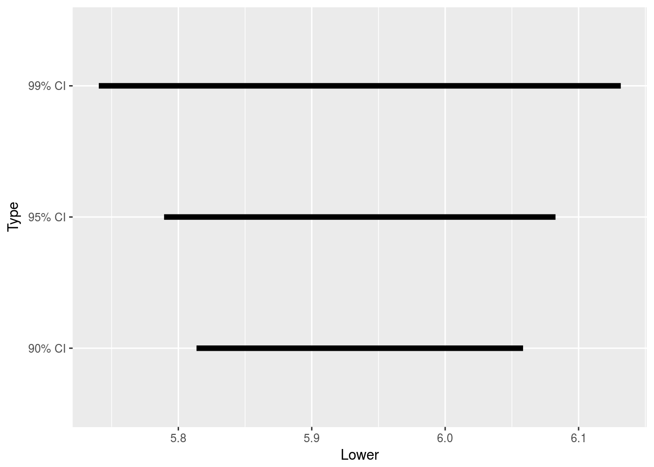
# It's clear that larger confidence levels lead to larger intervals, as can
# be seen in this graphic
Population Proportion, Single Sample
Suppose we collect categorical data, and encode observations that have some trait being tracked (“successes”) with 1, and the rest 0. This is a Bernoulli random variable, and our objective is to estimate the population proportion of successes, \(p\). The number of successes in the sample, \(\sum_{i = 1}^{n} X_i\), is a binomial random variable, and the natural estimator for the population proportion is the sample proportion, \(\hat{p} = \frac{1}{n}\sum_{i = 1}^{n} X_i\).
Computing a confidence interval for \(p\) has been revisited many times, each method trying to rectify faults of others (there is even an R package, binom, devoted to providing all the different methods for computing confidence intervals for the population proportion). A method that used to be popular, based on the Normal approximation for the distribution of the sample proportion \(\hat{p}\), is the confidence interval:
\[\hat{p} \pm z_{\frac{\alpha}{2}}\sqrt{\frac{\hat{p}(1 - \hat{p})}{n}} \equiv \left(\hat{p} - z_{\frac{\alpha}{2}}\sqrt{\frac{\hat{p}(1 - \hat{p})}{n}}; \hat{p} + z_{\frac{\alpha}{2}}\sqrt{\frac{\hat{p}(1 - \hat{p})}{n}}\right)\]
The function prop.test() will compute confidence intervals using this method, having the format prop.test(x, n), where x is the number of successes and n the sample size.
A June CNN-ORC poll found 420 individuals surveyed out of 1001 would vote for Donald Trump if the election were held that day. Let’s use this data to get a confidence interval for the proportion of voters who would vote for Trump.
prop.test(420, 1001)##
## 1-sample proportions test with continuity correction
##
## data: 420 out of 1001, null probability 0.5
## X-squared = 25.574, df = 1, p-value = 4.256e-07
## alternative hypothesis: true p is not equal to 0.5
## 95 percent confidence interval:
## 0.3888812 0.4509045
## sample estimates:
## p
## 0.4195804prop.test() found a confidence interval with a margin of error of roughly 3% (the target margin of error of the survey).
This confidence interval was popular in textbooks for years, but it is flawed to the point few advocate its use. The primary reason is that this interval is not guaranteed to capture the true \(p\) with the probability we specify, behaving erratically for different combinations of sample sizes and with more-or-less extreme \(p\). It’s thus considered unreliable, and alternatives are preferred.
The Hmisc package contains a function for computing confidence intervals for the population proportion, binconf(), that allows for a few other confidence intervals for the population proportion to be computed. The score-based method is advocated by the textbook author used in the lecture course, and is supported by binconf(). The interface of the function is different from the interface of similar functions in the stats (base R) package (it was not written by the same authors); instead of specifying conf.level, one specifies alpha in binconf(), with \(\alpha = 1 - C\) (the default value for alpha is .05, corresponding to a 95% confidence interval). Additionally, binconf() will not directly compute one-sided confidence bounds like prop.test() would. But otherwise usage is similar, with binconf(x, n, method = "wilson") computing a 95% confidence interval for a data set in which, out of n trials, there were x successes, using the score confidence interval.
Let’s use binconf() to compute the score confidence interval for the proportion of voters supporting Donald Trump, obtaining both a 95% and 99% confidence interval.
library(Hmisc)
# 95% CI
binconf(420, 1001, method = "wilson")
## PointEst Lower Upper
## 0.4195804 0.3893738 0.4504019# 99% CI
binconf(420, 1001, alpha = 0.01, method = "wilson")## PointEst Lower Upper
## 0.4195804 0.3800618 0.4601581The 95% confidence interval using the score method is not the same as the result from prop.test(), but not drastically different either.
binom.test() supports the exact confidence interval, which uses the CDF of the binomial distribution rather than a Normal approximation. The exact confidence interval can be computed via binom.test(x, n) (with all other common parameters such as conf.level and alternative being supported). binconf() also supports the exact confidence interval, where one merely sets method = "exact" to compute it.
binom.test(420, 1001)##
## Exact binomial test
##
## data: 420 and 1001
## number of successes = 420, number of trials = 1001, p-value =
## 4.029e-07
## alternative hypothesis: true probability of success is not equal to 0.5
## 95 percent confidence interval:
## 0.3887849 0.4508502
## sample estimates:
## probability of success
## 0.4195804# 99% confidence lower bound for Trump support, using binom.test
binom.test(420, 1001, alternative = "greater", conf.level = 0.99)##
## Exact binomial test
##
## data: 420 and 1001
## number of successes = 420, number of trials = 1001, p-value = 1
## alternative hypothesis: true probability of success is greater than 0.5
## 99 percent confidence interval:
## 0.3831763 1.0000000
## sample estimates:
## probability of success
## 0.4195804Paired Sample Confidence Interval for Difference in Means
Suppose you have paired data, \(X_i\) and a corresponding \(Y_i\). Examples of paired data include weight before (\(X_i\)) and after (\(Y_i\)) a weight-loss program, or the political views of a husband (\(X_i\)) and wife (\(Y_i\)). There are two different means for \(X_i\) and \(Y_i\), denoted \(\mu_X\) and \(\mu_Y\), and we want to know how these means compare.
Since the data is paired, we create a confidence interval using the differences of each \(X_i\) and \(Y_i\), \(D_i = X_i - Y_i\), and the confidence interval will describe the location of the mean difference \(\mu_D\). Thus, for paired data, after computing the differences, the procedure for computing a confidence interval is the same as the univariate case.
One approach for computing the confidence interval for the mean difference of paired data is with t.test(x - y), where x and y are vectors containing the paired data. Another approach would be to use t.test(x, y, paired = TRUE).
I illustrate by examining whether stricter enforcement of speed limit laws helps reduce the number of accidents. The Traffic data set (MASS) shows the effects of Swedish speed limits on accidents after an experiment where specific days in 1961 and 1962 saw different speed limits applied, in a paired study (days each year were matched). Thus a matched pairs design could be applied to see if the speed limit laws helped reduce accidents.
library(MASS)
library(reshape)
head(Traffic)
## year day limit y
## 1 1961 1 no 9
## 2 1961 2 no 11
## 3 1961 3 no 9
## 4 1961 4 no 20
## 5 1961 5 no 31
## 6 1961 6 no 26# The Traffic data set needs to be formed into a format that is more easily
# worked with. The following code reshapes the data into a form that allows
# for easier comparison of paired days
new_Traffic <- with(Traffic, data.frame(year = year, day = day, limit = as.character(limit),
y = as.character(y)))
melt_Traffic <- melt(new_Traffic, id.vars = c("year", "day"), measure.vars = c("limit",
"y"))
form_Traffic <- cast(melt_Traffic, day ~ year + variable)
form_Traffic <- with(form_Traffic, data.frame(day = day, limit_61 = `1961_limit`,
accidents_61 = as.numeric(as.character(`1961_y`)), limit_62 = `1962_limit`,
accidents_62 = as.numeric(as.character(`1962_y`))))
head(form_Traffic)## day limit_61 accidents_61 limit_62 accidents_62
## 1 1 no 9 no 9
## 2 2 no 11 no 20
## 3 3 no 9 no 15
## 4 4 no 20 no 14
## 5 5 no 31 no 30
## 6 6 no 26 no 23# Now we subset this data so that only days where speed limits were enforced
# differently between the two years
diff_Traffic <- subset(form_Traffic, select = c("accidents_61", "accidents_62",
"limit_61", "limit_62"), subset = limit_61 != limit_62)
head(diff_Traffic)## accidents_61 accidents_62 limit_61 limit_62
## 11 29 17 no yes
## 12 40 23 no yes
## 13 28 16 no yes
## 14 17 20 no yes
## 15 15 13 no yes
## 16 21 13 no yes# Get a vector for accidents when the speed limit was not enforced, and a
# vector for accidents for when it was
accident_no_limit <- with(diff_Traffic, c(accidents_61[limit_61 == "no"], accidents_62[limit_62 ==
"no"]))
accident_limit <- with(diff_Traffic, c(accidents_61[limit_61 == "yes"], accidents_62[limit_62 ==
"yes"]))
accident_limit## [1] 19 19 9 21 22 23 14 19 15 13 22 42 29 21 12 16 17 23 16 20 13 13 9
## [24] 10 27 12 7 11 15 29 17 17 15 25 9 16 25 25 16 22 21 17 26 41 25 12
## [47] 17 24 26 16 15 12 22 24 16 25 14 15 9accident_no_limit## [1] 29 40 28 17 15 21 24 15 32 22 24 11 27 37 32 25 20 40 21 18 35 21 25
## [24] 34 42 27 34 47 36 15 26 21 39 39 21 15 17 20 24 30 25 8 21 10 14 18
## [47] 26 38 31 12 8 22 17 31 49 23 14 25 24# It took a lot of work, but finally we have the data in a format we want.
# Now, the first thing I check is whether the differences are Normally
# distributed
qqnorm(accident_limit - accident_no_limit)
qqline(accident_limit - accident_no_limit)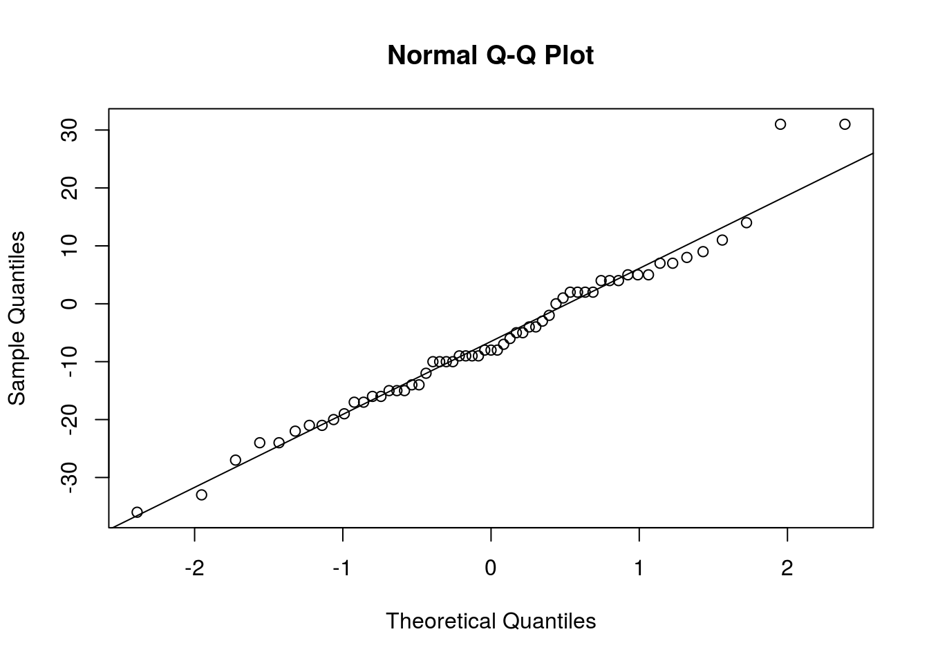
# Aside from a couple observations, the Normal distribution seems to fit
# very well. t procedures are safe to use.
t.test(accident_limit, accident_no_limit, paired = TRUE)
##
## Paired t-test
##
## data: accident_limit and accident_no_limit
## t = -3.7744, df = 58, p-value = 0.0003794
## alternative hypothesis: true difference in means is not equal to 0
## 95 percent confidence interval:
## -9.856470 -3.024886
## sample estimates:
## mean of the differences
## -6.440678The above analysis suggests that enforcing speed limits reduces the number of accidents, since zero is not in the interval.
Test for Difference in Population Means Between Two Samples
Analyzing paired data is simple since the analysis reduces to the univariate case. Two independent samples, though, are not as simple.
Suppose we have two independent data sets, with \(X_1, ..., X_n\) the first and \(Y_1, ..., Y_m\) the second, each drawn from two distinct populations. We typically wish to know whether the means of the two populations, \(\mu_X\) and \(\mu_Y\), differ. Thus, we wish to obtain a confidence interval for the difference in means of the populations, \(\mu_X - \mu_Y\).
The natural estimator for \(\mu_X - \mu_Y\) is \(\overline{X} - \overline{Y}\), so the point estimate of the difference is \(\bar{x} - \bar{y}\). The margin of error, though, depends on whether we believe the populations are homoskedastic or heteroskedastic. Homoskedastic populations have equal variances, so \(\sigma_X^2 = \sigma_Y^2\). Heteroskedastic populations, though, have different variances, so \(\sigma_X^2 \neq \sigma_Y^2\). Between the two, homoskedasticity is a much stronger assumption, so unless you have a reason for believing otherwise, you should assume heteroskedasticity. (It is the correct assumption the populations are, in fact, heteroskedastic, and if they are actually homoskedastic, the confidence interval should still be reasonably precise.)
For homoskedastic populations, the confidence interval is:
\[\bar{x} - \bar{y} \pm t_{\frac{\alpha}{2},n + m - 2}s\sqrt{\frac{1}{n} + \frac{1}{m}} \equiv \left(\bar{x} - \bar{y} - t_{\frac{\alpha}{2},n + m - 2}s\sqrt{\frac{1}{n} + \frac{1}{m}} ; \bar{x} - \bar{y} + t_{\frac{\alpha}{2},n + m - 2}s\sqrt{\frac{1}{n} + \frac{1}{m}}\right)\]
where \(s\) is the sample standard deviation of the pooled sample (that is, when \(X_1,...,X_n\) and \(Y_1,...,Y_m\) are treated as one sample).
Confidence intervals for heteroskedastic data are more complicated, since the \(t\) distribution is no longer the correct distribution to use to describe the behavior of the random variable from which the confidence interval is derived. That said, the \(t\) distribution can approximate the true distribution when the degrees of freedom used is:
\[\nu = \frac{\left(\frac{s_X^2}{n} + \frac{s_Y^2}{m}\right)^2}{\frac{\left(s_X^2/n\right)^2}{n - 1} + \frac{\left(s_Y^2/m\right)^2}{m - 1}}\]
with \(s_X^2\) and \(s_Y^2\) being the variances of the data sets \(x_1,...,x_n\) and \(y_1,...,y_m\), respectively. Then the confidence interval is approximately:
\[\bar{x} - \bar{y} \pm t_{\frac{\alpha}{2}, \nu}\sqrt{\frac{s_X^2}{n} + \frac{s_Y^2}{m}}\]
t.test() can compute confidence intervals in both these cases. The function call is similar to the case of paired data, though without setting paired = TRUE. Instead, set var.equal = TRUE for homoskedastic populations, and var.equal = FALSE (the default) for heteroskedastic populations.
Let’s illustrate this by determining whether orange juice or a vitamin C supplement increase tooth growth in guinea pigs (in the ToothGrowth data set).
# First, let's get the data into separate vectors
split_len <- split(ToothGrowth$len, ToothGrowth$supp)
OJ <- split_len$OJ
VC <- split_len$VC
# Gets CI for difference in means
t.test(OJ, VC)
##
## Welch Two Sample t-test
##
## data: OJ and VC
## t = 1.9153, df = 55.309, p-value = 0.06063
## alternative hypothesis: true difference in means is not equal to 0
## 95 percent confidence interval:
## -0.1710156 7.5710156
## sample estimates:
## mean of x mean of y
## 20.66333 16.96333# Is there homoskedasticity? Let's check a boxplot
boxplot(len ~ supp, data = ToothGrowth)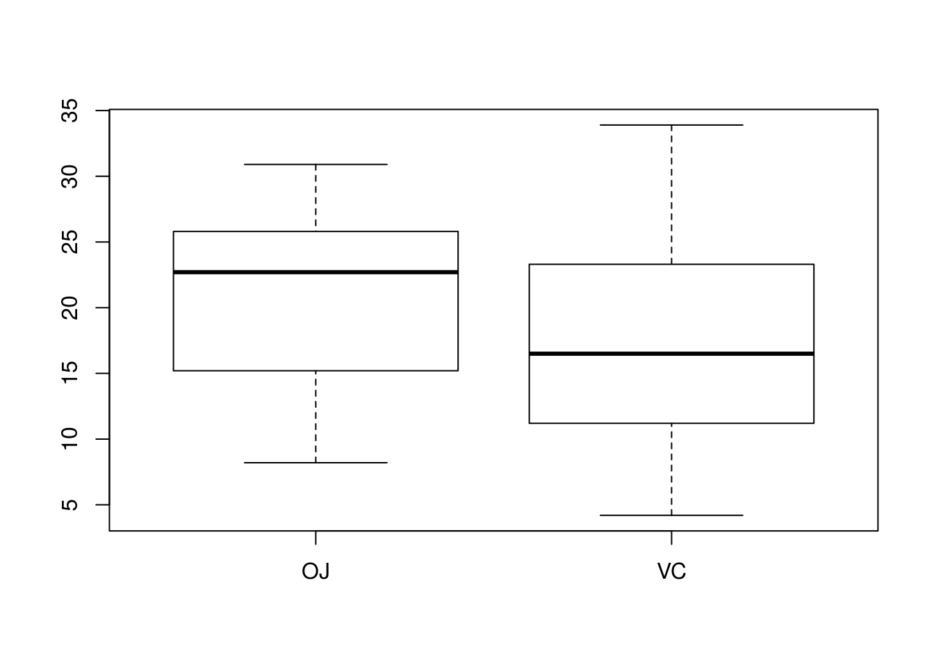
# These populations look homoskedastic; spread does not differ drastically
# between the two. A CI that assumes homoskedasticity is thus computed.
t.test(OJ, VC, var.equal = TRUE)
##
## Two Sample t-test
##
## data: OJ and VC
## t = 1.9153, df = 58, p-value = 0.06039
## alternative hypothesis: true difference in means is not equal to 0
## 95 percent confidence interval:
## -0.1670064 7.5670064
## sample estimates:
## mean of x mean of y
## 20.66333 16.96333# Not much changed (only slightly narrower).Difference in Population Proportions
If we have two populations, each with a respective population proportion representing the proportion of that population possessing some trait, we can construct a confidence interval for the difference in the proportions, \(p_X - p_Y\). The form of the confidence interval depends on which type is being used, and I will not discuss the details of how these confidence intervals are computed, but simply say that some of the functions we have seen for single sample confidence intervals, such as prop.test(), support comparing proportions (binconf() and binom.test() do not). The only difference is that rather than passing a single count and a single sample size to these functions, you pass a vector containing the count of successes in the two population, and a vector containing the two sample sizes (naturally they should be in the same order).
In the next example, I compare the proportions of men and women with melanoma who die from the disease.
mel_split <- split(Melanoma$status, Melanoma$sex)
# Get logical vectors for whether patient died from melanoma. Group 0 is
# women and group 1 is men, and the code 1 in the data indicates death from
# melanoma
fem_death <- mel_split[["0"]] == 1
man_death <- mel_split[["1"]] == 1
# Vector containing the number of deaths for both men and women
deaths <- c(Female = sum(fem_death), Male = sum(man_death))
# Vector containing sample sizes
size <- c(Female = length(fem_death), Male = length(man_death))
deaths/size
## Female Male
## 0.2222222 0.3670886# prop.test, with the 'classic' CLT-based CI
prop.test(deaths, size)##
## 2-sample test for equality of proportions with continuity
## correction
##
## data: deaths out of size
## X-squared = 4.3803, df = 1, p-value = 0.03636
## alternative hypothesis: two.sided
## 95 percent confidence interval:
## -0.283876633 -0.005856138
## sample estimates:
## prop 1 prop 2
## 0.2222222 0.3670886