Lecture 1
R Basics
Using R as a Calculator
Lots of work in R is done via the interpreter. You can use the interpreter as a calculator, and thus can do some simple calculations.
# Some basic arithmetic
2 + 2
## [1] 41 - 7## [1] -62 * 3## [1] 6(1 + 1) * 3## [1] 62^3## [1] 810/2## [1] 5# One can also use functions for more advanced calculations
sqrt(9)## [1] 3exp(3)## [1] 20.08554# A familiar built-in value
pi## [1] 3.141593When using a computer as a calculator, though, you may observe behavior that seems… strange.
# Be aware that any time you use computers for calculation you may get the
# 'wrong' answer. This is due to floating-point arithmetic and how computers
# see numbers.
sqrt(2)^2
## [1] 2# What's this?
sqrt(2)^2 - 2## [1] 4.440892e-16(For an explanation of this phenomenon, watch this video by Computerphile on floating-point numbers.)
Obviously, though, we want to use R for more than a glorified calculator.
Variables
As with any programming language, R can store information in variables. R has a few ways to store variables, with the <-, ->, and = operators (there are a few others that I won’t discuss here).
# One way to create a variable
var1 <- 1
# Another way to create a variable
var2 = 2
# A third way, this time where the variable is on the RIGHT side of the
# assignment operator!
var3 <- 3
# What do you get?
var1 + var2
## [1] 3var2 * var3## [1] 6There are rules as to how variables can be named. In addition to not being reserved words, they can only use alpha-numeric characters (letters and numbers), or the _ or . characters. Also, they cannot begin with a number (so while var1 is legal, 1var is not). Variables are case-sensitive; var1 is not the same as Var1 or VAR1.
# These are all valid names for variables
var1 <- 10
variable_number_2 <- 20
variable.number.3 <- 30  # <---- I would suggest avoiding this style of variable naming, though; use '_' instead
variableNumber4 <- 40

# None of these are the same
var1 <- 10
Var1 <- 230
VAR1 <- -5


var1 + 1
## [1] 11Var1 + 1## [1] 231VAR1 + 1## [1] -4As a side note, notice that a line break will usually begin a new command. This is not always true! If a command is not finished from R’s perspective, it will see the contents of the next line as being part of the same command. This can sometimes be confusing, while other times it can be used to your advantage. Furthermore, you can use the ; character to separate commands on the same line, or explicitly end a command like in C-based programming languages like C, C++, or Java (though this is usually not done). Aside from this, R generally ignores white space (space, tabs, new lines, etc.).
# Because there is nothing after the '+' on the first line, R looks for the
# rest of the command on the second line.
5 +
5
## [1] 10# It could even be a few lines down! (DON'T EVER DO THIS!!!!)
10 +
1## [1] 11R variables are untyped, but that does not mean that the object they reference is untyped. Some basic types you will encounter early (and there are many, many others) include:
- Numeric, like
124or3.14159 - Character, like
"hello bobby"or"124"or'cmiller@math.utah.edu' - Boolean, either
TRUEorFALSE - Vectors, which are a collection of objects of all the same type
- Functions, which you can think of as being a “mini program”, like
log,sqrt,mean, orhelp - Data frames, which store datasets in memory in a tabular format
# A numeric variable
num_var <- 124
# Character data
char_var <- "hello"
# Boolean
bool_var <- TRUE
# A vector of data
data_vec <- c(1, 20, 6, 2)
# Another vector of data
data_vec2 <- c("hello", "world")

# There are functions for type checking
not_a_number <- "124"
is.numeric(not_a_number)
## [1] FALSEis.character(not_a_number)## [1] TRUE# Sometimes you can force a variable of one type to be another type.
is_a_number <- as.numeric(not_a_number)
is.numeric(is_a_number)## [1] TRUEPackages
The true power of R is in its packages. R has an ever-growing community of users and developers, many of whom write free packages to extend R’s functionality. These packages are made available to all R users on websites like CRAN (the Comprehensive R Archive Network) or GitHub.
Packages from CRAN are easily downloaded and installed using the install.packages() function, like so:
# Install the "UsingR" package for Verzani's book
install.packages("UsingR")
Once you install a new package, you can load it into the R environment using require() or library().
library(UsingR)
# Alternatively, you could use require("UsingR")
Today there are well over 7000 packages on CRAN alone, and this growth is likely to continue.
Data sets
Datasets in R are usually stored in vectors (for univariate data) or data frames (for multivariate data). For now, we will work with built-in data sets or those included in packages. If a dataset isn’t already in the R environment but does exist in some package, it can be brought in using the data() function. The head() function allows us to view only a few observations from a dataset (in order to prevent our screen from being flooded with all the data), and the str() function gives us a further description of the dataset.
# Let's load in a univeriate dataset containing the lengths of major North
# American rivers
data(rivers)
# We can see a few of the observations to get a glimpse at the nature of the
# data.
head(rivers)
## [1] 735 320 325 392 524 450# We can see more information via str()
str(rivers)## num [1:141] 735 320 325 392 524 ...# Just for fun, what is the combined length of all these rivers?
sum(rivers)## [1] 83357# Let's have even more fun by seeing what proportion of this total length
# each river accounts for.
rivers/sum(rivers)## [1] 0.008817496 0.003838910 0.003898893 0.004702664 0.006286215
## [6] 0.005398467 0.017503029 0.001619540 0.005578416 0.007197956
## [11] 0.003958876 0.004030855 0.003359046 0.003778927 0.010437036
## [16] 0.010868913 0.002423312 0.003946879 0.003479012 0.011996593
## [21] 0.007197956 0.006058279 0.017395060 0.010077138 0.014911765
## [26] 0.010676968 0.004198808 0.004882613 0.003431026 0.003359046
## [31] 0.006298211 0.008637547 0.004678671 0.002999148 0.003922886
## [36] 0.002759216 0.003179097 0.010197104 0.002519285 0.007557854
## [41] 0.003119114 0.002759216 0.004318773 0.008757513 0.007197956
## [46] 0.003670957 0.004678671 0.005038569 0.003491009 0.008517581
## [51] 0.004078842 0.002603261 0.003371043 0.004222801 0.003107118
## [56] 0.002999148 0.005638399 0.008157683 0.006838058 0.004198808
## [61] 0.003598978 0.006718092 0.010796934 0.007497871 0.003982869
## [66] 0.028168000 0.014048010 0.044507360 0.027772113 0.030387370
## [71] 0.009357343 0.003359046 0.004918603 0.005518433 0.003119114
## [76] 0.003059131 0.005170532 0.004198808 0.009117411 0.007413894
## [81] 0.004054848 0.011768658 0.015667550 0.005998296 0.008349629
## [86] 0.007257939 0.002999148 0.004930600 0.012644409 0.008817496
## [91] 0.002795206 0.005218518 0.005878331 0.003718944 0.005518433
## [96] 0.004594695 0.004498722 0.015235673 0.006538143 0.005338484
## [101] 0.022613578 0.004558705 0.003598978 0.004558705 0.004522716
## [106] 0.005098552 0.003311060 0.002519285 0.009597274 0.005038569
## [111] 0.004198808 0.004318773 0.006454167 0.013196252 0.014455895
## [116] 0.003766930 0.002843193 0.007317922 0.004318773 0.006478160
## [121] 0.012452464 0.005086555 0.003718944 0.003598978 0.005326487
## [126] 0.003610974 0.003215087 0.007437888 0.002579267 0.007821779
## [131] 0.010796934 0.006298211 0.002951162 0.004318773 0.006346198
## [136] 0.005998296 0.008637547 0.003239080 0.005158535 0.008049714
## [141] 0.021233970# Let's look at our first ever data frame, the famous iris dataset
head(iris)## Sepal.Length Sepal.Width Petal.Length Petal.Width Species
## 1 5.1 3.5 1.4 0.2 setosa
## 2 4.9 3.0 1.4 0.2 setosa
## 3 4.7 3.2 1.3 0.2 setosa
## 4 4.6 3.1 1.5 0.2 setosa
## 5 5.0 3.6 1.4 0.2 setosa
## 6 5.4 3.9 1.7 0.4 setosastr(iris)## 'data.frame': 150 obs. of 5 variables:
## $ Sepal.Length: num 5.1 4.9 4.7 4.6 5 5.4 4.6 5 4.4 4.9 ...
## $ Sepal.Width : num 3.5 3 3.2 3.1 3.6 3.9 3.4 3.4 2.9 3.1 ...
## $ Petal.Length: num 1.4 1.4 1.3 1.5 1.4 1.7 1.4 1.5 1.4 1.5 ...
## $ Petal.Width : num 0.2 0.2 0.2 0.2 0.2 0.4 0.3 0.2 0.2 0.1 ...
## $ Species : Factor w/ 3 levels "setosa","versicolor",..: 1 1 1 1 1 1 1 1 1 1 ...# You can think of this as being a table or matrix. In fact, it's a
# combination of equal-length vectors. We can get the Sepal.Length vector
# using the $ operator
iris$Sepal.Length## [1] 5.1 4.9 4.7 4.6 5.0 5.4 4.6 5.0 4.4 4.9 5.4 4.8 4.8 4.3 5.8 5.7 5.4
## [18] 5.1 5.7 5.1 5.4 5.1 4.6 5.1 4.8 5.0 5.0 5.2 5.2 4.7 4.8 5.4 5.2 5.5
## [35] 4.9 5.0 5.5 4.9 4.4 5.1 5.0 4.5 4.4 5.0 5.1 4.8 5.1 4.6 5.3 5.0 7.0
## [52] 6.4 6.9 5.5 6.5 5.7 6.3 4.9 6.6 5.2 5.0 5.9 6.0 6.1 5.6 6.7 5.6 5.8
## [69] 6.2 5.6 5.9 6.1 6.3 6.1 6.4 6.6 6.8 6.7 6.0 5.7 5.5 5.5 5.8 6.0 5.4
## [86] 6.0 6.7 6.3 5.6 5.5 5.5 6.1 5.8 5.0 5.6 5.7 5.7 6.2 5.1 5.7 6.3 5.8
## [103] 7.1 6.3 6.5 7.6 4.9 7.3 6.7 7.2 6.5 6.4 6.8 5.7 5.8 6.4 6.5 7.7 7.7
## [120] 6.0 6.9 5.6 7.7 6.3 6.7 7.2 6.2 6.1 6.4 7.2 7.4 7.9 6.4 6.3 6.1 7.7
## [137] 6.3 6.4 6.0 6.9 6.7 6.9 5.8 6.8 6.7 6.7 6.3 6.5 6.2 5.9Help
R has many, many functions. In 2014, there were approximately 182,393 R functions that could be used (most of them in packages). There is no way anyone could remember all of them.
Fortunately, it’s easy to access documentation in R, especially if you are using RStudio. The help() function will look up documentation for a string entered. This is made even easier by just typing ? and the name of the package/function/dataset you want to see documentation for.
# Here's how to access the documentation of the mean() function
help("mean")
# Or even easier:
?mean
Univariate Data Analysis
Vectors
Univariate data is usually stored as vectors. The most basic function for creating a vector is the c() function, where the arguments of the function (separated by commas) become the contents of the vector. It generally doesn’t matter what the type of data the contents of the vector are so long as they are all the same.
# A numeric vector of fictitious data
num_vec <- c(10, 13, -1, 0.02, 0, -3.31)
# A vector of character data
char_vec <- c("joe", "phil", "jan", "denise", "tom")
# A vector of boolean values
bool_vec <- c(TRUE, TRUE, FALSE)
# A vector of functions? WHAT IS THIS MADNESS?
func_vec <- c(mean, sum, sd)
# But this does not create a vector of vectors; all vectors are flattened into one vector (it is possible to make a vector of vectors, but it's tricky)
not_a_vec_of_vecs <- c(c(1,2,3),c(4,54),c(10,2,-6))

# If I want to see the contents of a vector, just type its name into the interpreter
not_a_vec_of_vecs
## [1] 1 2 3 4 54 10 2 -6If you don’t specify the type of data you are storing in a variable, or if one has not already been assigned, R will think it’s a vector.
im_a_vector <- 5
is.vector(im_a_vector)
## [1] TRUETo access the contents of a vector, you can use [] notation, like vec[x]. x identifies the elements of the vector you want. This is called indexing.
Some notes about x:
- Items in a vector can always be found via an integer.
vec[1]will get the first element of the vector, andvec[5]the fifth. Also, instead of specifying what indices you do want, you can specify the indices you don’t want with negative integers. For example,vec[-1]isvecwith all except forvec[1].vec[0]is an empty vector that is of the same type asvec. - Some vectors have named elements. In that case, you can access elements of the vector by name, using a character string. For example, if
citiesis a vector of city populations which is indexed with city names,cities["Salt Lake City"]will find the population of Salt Lake City in the vector. If you want to see the names of the elements, use thenames()function. (Not surprisingly, the object returned bynames()is also a vector, specifically a character vector.) xcan be another vector, and thus you can index a vector with another vector so long as the values contained inxare a valid means of indexing. We could index a vector withvec[c(1,2,3)]orcities[c("Salt Lake City", "Provo")].xcould be a vector of booleans. EveryTRUEinxwill lead to the element inveccorresponding to where theTRUEis located inxwill be included, and every element invecwherexisFALSEwill not be included. (While this implies thatxmust be the same length asvec, this is not necessarily true; ifxis shorter, the contents ofxwill be recycled until R has made a decition for each element ofvecwhether to include it or not. I discuss recycling more later.)vec[]will return the entire vectorvec. This is sometimes useful.
# You can assign names to elements using name = value notation in c()
friendly_vector <- c(jon = 1, tony = 4, janet = 5)
names(friendly_vector)
## [1] "jon" "tony" "janet"friendly_vector[1]## jon
## 1friendly_vector[c(2,3)]## tony janet
## 4 5friendly_vector[-2]## jon janet
## 1 5friendly_vector["tony"]## tony
## 4friendly_vector[c("jon", "tony")]## jon tony
## 1 4friendly_vector[c(TRUE, TRUE, FALSE)]## jon tony
## 1 4# You can rename elements in a vector like so:
names(friendly_vector) <- c("jack", "jill", "dick")
friendly_vector["jack"]## jack
## 1You can also use indexing to change the values of a vector, or even expand it. vec[x] <- val will replace the contents of vec at x with val if val is the same type as the rest of the data in vec and x is any valid means of indexing vec. x could consist of indices that do not already exist in vec, in which case those indices will be added to vec, thus expanding it. If x consists of integer indices outside the range of existing integer indices, these other indices will be created as well and filled with NA’s.
You can also delete values from the vector with vec[x] <- NULL
# friendly_vector was defined in an earlier code block
# Change existing values
friendly_vector["jack"] <- 16
friendly_vector[2] <- 19
friendly_vector
## jack jill dick
## 16 19 5# Adding new values
friendly_vector[4] <- 21
friendly_vector## jack jill dick
## 16 19 5 21friendly_vector["danielle"] <- 0
friendly_vector## jack jill dick danielle
## 16 19 5 21 0friendly_vector[c(6, 7, 8)] <- 12
friendly_vector## jack jill dick danielle
## 16 19 5 21 0 12 12 12friendly_vector[20] <- 18While vectors must contain data of one type, there is a special type that can be included in any vector: NA. This value represents “missing information”. NA isn’t like other values and needs to be handled with care. The function is.na() identifies these values in vectors.
not_finished <- c(1, 4, 5, NA, 2, 2)
not_finished
## [1] 1 4 5 NA 2 2# If I want to access the non-NA parts of the vector, I can do so like this
not_finished[!is.na(not_finished)]## [1] 1 4 5 2 2There are other special types in R resembling but dfferent from NA. NULL is a lot like NA but usually means that something in R is unavailable (whereas NA is more akin to missing data in a dataset). Inf and -Inf are special values denoting infinity and negative infinity respectively. These are, in some sense, numeric, and represent values that are very large (or very small, in the case of -Inf), and can occur when dividing non-zero numbers by zero. NaN effectively means “not a number”, and occurs when some numerical error occurs, like dividing zero by zero. Again, these cases must be handled with care, and there are special functions like is.na() for detecting them in vectors.
There are other ways to create vectors other than with the c() function. Some common ways are listed below:
- The
:constructor can be used to create sequences. For example,1:10will create a vector of numbers from 1 to 10, incrementing by 1.10:0creates a vector starting at 10 and ending at 0, decrementing by 1. You can also replace the endpoints with variables, or expressions in parentheses, like1:nor1:(2 + 2). - Sometimes you may want to create a sequence but want more control over incrementation, or how many elements in the vector you want. In this case, use the
seq()function. You can make a sequence of numbers incrementing by 2 going from 1 to 100 withseq(1, 100, by = 2), or a sequence of numbers between 0 and 1 with length 100 withseq(0, 1, length = 100). (Seehelp("seq")to see all the many ways to create sequences withseq().) - The
rep()function can make vectors with repeating elements. Let’s say I want to repeat the character values “"a","b", and"c"three times total. I can do so withrep(c("a", "b", "c"), times = 3). Alternatively, if I wanted to repeat these values each three times, I would do so withrep(c("a", "b", "c"), each = 3). (Seehelp("rep")to see all the many ways to create sequences withrep().) - Sometimes I want to create character vectors where I have pasted together strings from separate vectors. For example, if I want a character vector containing the names of one hundred treatments, it may be tedious to type
c("Treatment 1", "Treatment 2", ..., "Treatment 100"). Thepaste()function makes this much easier. I can create such a vector withpaste("Treatment", 1:100); each of the elements from both vectors will be pasted together into a new vector. By default, these elements will be separated with a space character, but I can change this behavior by specifying thesepparameter inpaste(). For example, if I want"Treatment_1"rather than"Treatment 1", I can do so withpaste("Treatment", 1:100, sep = "_").
I demonstrate these techniques below.
# Create a vector of numbers from 1 to 10
1:10
## [1] 1 2 3 4 5 6 7 8 9 10# In reverse
10:1## [1] 10 9 8 7 6 5 4 3 2 1# Getting creative
1:(2 + 2)## [1] 1 2 3 4# Another way to make a sequence
seq(-1, 1, by = 0.5)## [1] -1.0 -0.5 0.0 0.5 1.0# Yet another way to make a sequence
seq(0, 20, length = 3)## [1] 0 10 20# A repeating sequence of letters
rep(c("a", "b", "c"), times = 3)## [1] "a" "b" "c" "a" "b" "c" "a" "b" "c"# A sequence of repeating letters
rep(c("a", "b", "c"), each = 3)## [1] "a" "a" "a" "b" "b" "b" "c" "c" "c"# A quick way to make a character vector
paste("Treatment", 1:5)## [1] "Treatment 1" "Treatment 2" "Treatment 3" "Treatment 4" "Treatment 5"You can do mathematical operations with vectors, such as +, -, *, /, ^, and others. Operations are often applied component-wise, using R’s recycling behavior. Recycling occurs when two vectors are not of equal length. Let’s say you have a vector vec1 that is longer than vec2, and you do an operation such as vec1 + vec2. Let’s say length(vec1) == 12 and length(vec2) == 4. At first, the resulting vector will add, component-wise, each element from each vector; think vec1[1] + vec2[1], vec1[2] + vec2[2], vec1[3] + vec2[3], and vec1[4] + vec2[4]. After the fourth index, though, there are no more elements in vec2, so R will start from the beginning of vec2 and keep going, resulting in vec1[5] + vec2[1], vec1[6] + vec2[2], and so on. R will continue to do this until it has reached the end of vec1. You would get the same result for vec2 + vec1; it doesn’t matter which side of + has the longer vector. If the longer vector is not a multiple of the shorter vector, though, R will throw a warning message.
vec1 <- c(0, 0, 10, -1, 5, 6)
# R treats "1" as a vector of length 1, and thus recycles
vec1 + 1
## [1] 1 1 11 0 6 7vec1 * 2## [1] 0 0 20 -2 10 12vec1 ^ 2## [1] 0 0 100 1 25 36vec2 <- 1:2
# Another case of recycling behavior
vec1 + vec2## [1] 1 2 11 1 6 8# Same result if I switch the order
vec2 + vec1## [1] 1 2 11 1 6 8# R will complain if the length of the longer vector is not a multiple of the length of the shorter object, though it will still produce a result
vec1 / 1:4## Warning in vec1/1:4: longer object length is not a multiple of shorter
## object length## [1] 0.000000 0.000000 3.333333 -0.250000 5.000000 3.000000vec1 ^ vec2## [1] 0 0 10 1 5 36# Does NOT get same result because ^ is not commutative
vec2 ^ vec1## [1] 1.0 1.0 1.0 0.5 1.0 64.0Of course, when working with vectors of the same length, recycling isn’t a concern.
# These vectors are the same length, so no need to worry about recycling
vec1 <- 1:3
vec2 <- 10:12
vec1 + vec2
## [1] 11 13 15vec1 * vec2## [1] 10 22 36vec1 ^ vec2## [1] 1 2048 531441# That said, it's not hard to guess what will happen when one of the objects is length one (like a vector)
(1:10) ^ 2 # First ten squares## [1] 1 4 9 16 25 36 49 64 81 1002 ^ (1:10) # First ten powers of two## [1] 2 4 8 16 32 64 128 256 512 1024Recycling occurs elsewhere in R. We saw recycling behavior when indexing a vector with a vector of booleans earlier. There are other instances in R as well.
Some functions are vector-valued. For example, when passed a vector, sqrt() will take the square root of every element in the vector.
vec <- 1:5
sqrt(vec)
## [1] 1.000000 1.414214 1.732051 2.000000 2.236068exp(vec)## [1] 2.718282 7.389056 20.085537 54.598150 148.413159vec[3] <- NA
# Creates a vector of booleans
is.na(vec)## [1] FALSE FALSE TRUE FALSE FALSEAnother important set of operators are logical operators, which return boolean data. Such operators include:
==: This detects equality (notice that this is not=, which is an assignment operator). If or when the object on the left equals the object on the right, the result will beTRUE; otherwise, it will beFALSE. For vectors, this does not return whether the two vectors are identical, but when one vector is equal to the other component-wise.<and>: These detects “less” or “greater than”, like in mathematics. This is intended for numeric data, but can be used for other types of data as well (although rarely, and probably not well).<=and>=: These detect “less than or equal to” or “greater than or equal to”.!=: This detects “not equal to”, and is the opposite of==.&: This is logical “and”, and is true when the boolean or statment on the left is true and the boolean or statement on the right is true. Thus,(1 == 1) & (2 >= 1) == TRUEand(1 == 2) & (2 >= 1) == FALSE.|: This is logical “or”, and is true when the boolean or statement on the left is true or the boolean or statement on the right is true. Thus,(1 == 1) | (2 >= 1) == TRUEand(1 == 2) | (2 >= 1) == TRUE.!: This is logical “not”, negating any truth statement. So!TRUE == FALSEand!(1 == 2) == TRUE.%in%: This logical operator is unique compared to the others considered here, since this is actually a function. The argument on the right-hand side of this operator must be a vector, and this operator whether elements on the left-hand side are in the vector on the right-hand side (in logic, this is \(x \in S\) where \(S\) is a set). Thus,3 %in% c(1,2,3) == TRUEand3 %in% c(1, 2) == FALSE.
Like other operators, these utilize recycling and may return vectors. Examples are shown below.
vec1 <- c(1, 4, 21, 22, -5)
vec2 <- c(1, 2, 3, 4, -5)
# True only in the first and last positions
vec1 == vec2
## [1] TRUE FALSE FALSE FALSE TRUEvec1 < 4 # True for first and last elements## [1] TRUE FALSE FALSE FALSE TRUEvec2 <= 4 # True in first, second, and last elements## [1] TRUE TRUE TRUE TRUE TRUE!(vec1 <= 4) # Inverse of above## [1] FALSE FALSE TRUE TRUE FALSE# %% is the modulus operator, returning the remainder when the number on the
# left is divided by the number on the right. vec1 %% 2 == 0 is a way to
# detect even numbers (since the remainder when dividing an even number by 2
# must be zero).
(vec1 > 20) & !(vec1%%2 == 0) # Only true in third position## [1] FALSE FALSE TRUE FALSE FALSE(vec1 > 20) | !(vec1%%2 == 0) # Not true in second or fourth## [1] TRUE FALSE TRUE TRUE TRUE1:4 %in% vec1 # One and four are in vec1## [1] TRUE FALSE FALSE TRUE# Some useful functions are the any() and all() functions, which take
# boolean vectors as arguments and return whether anywhere the vector is
# true or whether the vector is true everywhere, respectively. In other
# words, any() will 'or' all elements of the vector, and all() will 'and'
# all elements in the vector.
any(1:4 %in% vec1) # Is there a number between 1 and 4 in vec1?## [1] TRUEall(1:4 %in% vec1) # Are all numbers between 1 and 4 in vec1?## [1] FALSEMany other functions return logical data, notably the is.object() family of functions like is.vector() or is.na().
While a vector of booleans for when a condition is true is nice, sometimes you may not want whether a statement is true for each element of a vector, but for which elements of a vector a statement is true. In this case, the which() function will tell you the indices of where an input vector is TRUE.
which(c(TRUE, FALSE, FALSE, TRUE, FALSE))## [1] 1 4which(15:25 > 20)## [1] 7 8 9 10 11# I'm going to create a dataset with NA's, and use which() to find the NA's
# and also the 'good' data
data_vec <- 1:100
data_vec[c(21, 33, 49, 61, 62)] <- NA
which(is.na(data_vec)) # Where are the NA's## [1] 21 33 49 61 62which(!is.na(data_vec)) # Where is the non-NA data?## [1] 1 2 3 4 5 6 7 8 9 10 11 12 13 14 15 16 17
## [18] 18 19 20 22 23 24 25 26 27 28 29 30 31 32 34 35 36
## [35] 37 38 39 40 41 42 43 44 45 46 47 48 50 51 52 53 54
## [52] 55 56 57 58 59 60 63 64 65 66 67 68 69 70 71 72 73
## [69] 74 75 76 77 78 79 80 81 82 83 84 85 86 87 88 89 90
## [86] 91 92 93 94 95 96 97 98 99 100# How much data is NA?
length(which(is.na(data_vec)))## [1] 5# Alternatively, I can sum a boolean vector to find the same answer (FALSE
# is treated as 0 and TRUE as 1)
sum(is.na(data_vec))## [1] 5A special type of vector not discussed earlier is a factor vector, which is similar to a character vector but requires that each value of the vector be in a list of levels, which describe the values a factor vector can take. (R also views vactors differently internally than character vectors.) Factor vectors are thus used for storing categorical data. You can create a factor with the factor() function.
When manipulating factor data, there is an additional restriction to the ones discussed already: you cannot add a value that is not in the levels of the factor (aside from NA). You would have to add the value to the levels of the factor first, then add the value. Also, beware that changing the levels will also change the values stored in the factor. You can set the levels of a factor with levels(x) <- y, where x is the factor vector and y a vector representing the new levels of the factor.
# Create a factor of color data
color_data <- c("blue", "red", "blue", "blue", "blue", "red", "red", "blue")
# Create the factor, declaring the levels; notice that I included a category
# that is not in the data vector
colcat1 <- factor(color_data, levels = c("red", "green", "blue"))
colcat1
## [1] blue red blue blue blue red red blue
## Levels: red green blue# If I do not declare the levels, R will use the values stored in the vector
# to guess what they are
colcat2 <- factor(color_data)
# Now I change data; for the first, no complaint if I add 'green'
colcat1[1] <- "green"
colcat1## [1] green red blue blue blue red red blue
## Levels: red green blue# But 'green' is not in the levels of colcat2, so an warning is issued and
# NA is added instead
colcat2[1] <- "green"## Warning in `[<-.factor`(`*tmp*`, 1, value = "green"): invalid factor level,
## NA generatedcolcat2## [1] <NA> red blue blue blue red red blue
## Levels: blue red# I can see the levels of these with levels()
levels(colcat1)## [1] "red" "green" "blue"levels(colcat2)## [1] "blue" "red"# I can rearrange all the categories by changing the levels
levels(colcat1) <- c("blue", "red", "green")
colcat1## [1] red blue green green green blue blue green
## Levels: blue red green# Here I add a new level to those specified for colcat2
levels(colcat2)[3] <- "green"
# Now I can add 'green' to colcat2 without complaint
colcat2[1] <- "green"
colcat2## [1] green red blue blue blue red red blue
## Levels: blue red greenFunctions
Functions are one of the most important objects in R. In fact, R follows a programming paradigm called functional programming, where most operations are seen as the evaluation of functions. You can think of functions as miniature programs for performing certain tasks.
In R, functions have two parts:
Arguments are the values passed to the function for evaluation. In the statement
f(x, y), the variables between the parentheses,xandy, are the arguments of the function. A function will typically expect an argument to be of a particular type and may throw an error when that type is not received, but the expected type could be anything from a vector to a data frame to even another function. Some functions have many arguments but have default values assigned to most of them so that the user specifies those arguments only if they wish to change the function’s default behavior.The body of a function is the part of the function that performs computations (involving the parameters) and possibly returning an output. The output of the function is either the last value computed (and not assigned to a variable) or a value returned by the
return()function.
To create a named function, use the syntax my_func <- function(arguments) { function body }. Below I create a function.
# Let's create a function that returns the length of the longest vector
# passed to it. It will take two vectors x and y as arguments, and return
# the length of the longer vector
longest_length <- function(x, y) {
    l1 <- length(x)  # This is a local variable that will be visible only in the function, not the rest of R
    l2 <- length(y)
    max(l1, l2)  # This is the last unevaluated computation and thus is returned by the function
}
# Note that longest_length is a variable storing a function, and
# longest_length() is a function call

# Testing it out
vec1 <- c("bob", "jim", "margaret", "danny")
vec2 <- c(22, -9)
longest_length(vec1, vec2)
## [1] 4# Functions will check the position of objects passed and assign them to the
# arguments in the same position in the function definition. Alternatively
# (and very useful when there are many arguments not all of which are
# specified), you can use = to set specific arguments by name.
longest_length(y = vec2, x = vec1)## [1] 4Functions are extremely important objects in R and the key to R programming. Appendix A of the Verzani textbook discusses function programming in more detail.
Visually Exploring a Dataset
R has many techniques built-in for visually analyzing datasets, and many packages that do so even better, such as the very popular ggplot2 package (I used ggplot2 for all the graphics for my first report on Utah’s gender gap in wages written for Voices for Utah Children, which you can read here). Here I will discuss how to make a few basic graphics for visually analyzing a dataset.
Stem-and-leaf plot
Use the stem() function to create a stem-and-leaf plot.
stem(rivers)##
## The decimal point is 2 digit(s) to the right of the |
##
## 0 | 4
## 2 | 011223334555566667778888899900001111223333344455555666688888999
## 4 | 111222333445566779001233344567
## 6 | 000112233578012234468
## 8 | 045790018
## 10 | 04507
## 12 | 1471
## 14 | 56
## 16 | 7
## 18 | 9
## 20 |
## 22 | 25
## 24 | 3
## 26 |
## 28 |
## 30 |
## 32 |
## 34 |
## 36 | 1The display suggests that the rivers dataset is very right-skewed. Let’s see if this agrees with other plots.
Dotplot
You can use stripchart() to make dotplots. The default behavior of this function doesn’t produce a very useful plot (truth be told, plotting functions in other packages make better dotplots in general than stripchart()), so set method = "stack" to enable stacking. I also set pch = 20 to change the plotting character used from the default square to a filled-in circle, which is easier to read.
Many R plotting functions have parameters main, xlab, and ylab. These are so you set the title of the plot, and the names of the labels. I do so in the plot I create as well.
# Make a dotplot of the rivers data
stripchart(rivers, method="stack", pch = 20,
           # Adding axis labels
           main = "Length of North American Rivers",
           xlab = "Length")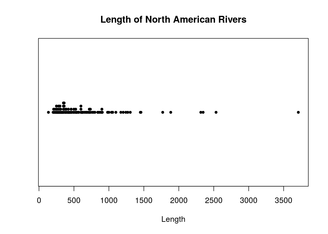
The rivers dataset is slightly large, with 141 observations. The plots used so far may not result in very good graphics for datasets like this. I next consider graphics that may handle larger datasets better.
Histogram
The hist() function creates histograms in R. Calling hist(x) for some dataset x will create a histogram R thinks is appropriate. R will automatically choose classes and the number of classes to used based on built-in algorithms. I show an example below:
hist(rivers)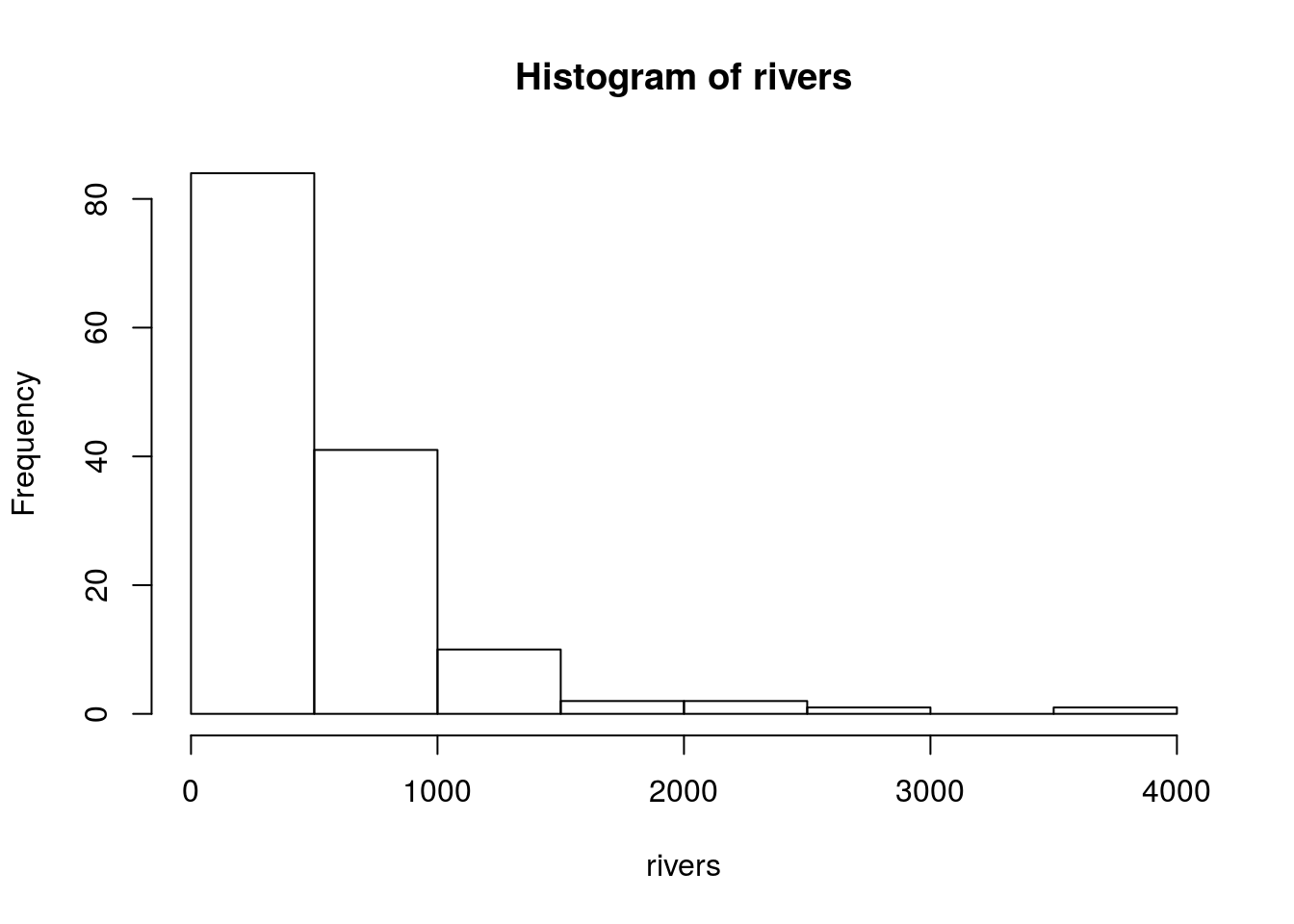
We can change the parameters of the hist() function to have more control over the result. For example:
R automatically chooses axis names and the main title, which usually are not very good names. We can change these defaults to reasonable labels by setting the
main,xlab, andylabparameters.By default, R will plot the frequency rather than the relative frequency of each class. The result is indistinguishable until you wish to overlay a histogram with a smooth curve or otherwise be more creative with the chart. Set
freq = FALSEto show relative frequencies, or probabilities.R creates left-inclusive histograms by default. If we want right-inclusive histograms, set
right = TRUE.The
breaksparameters is used for setting where the break points are located. If we setbreaksto an integer, this will tell R how many classes to use. For example, if we want \(\sqrt{n}\) classes for theriversdataset, we can do so by settingbreaks = round(sqrt(length(x))). (That said, the method R uses for determining how many classes to use is usually better than the \(\sqrt{n}\) rule.)Do we really like white bars in our histogram? The
colparameter can change their color. For example, setcol = "gray"for gray bars.
There are many more parameters for the hist() function than this; I invite you to read the function’s documentation for more details. Here is another histogram for the rivers dataset, this one changing some parameters.
hist(rivers, main = "Distribution of the Lengths of Major North American Rivers",
     xlab = "Length of River",
     freq = FALSE,
     right = TRUE,
     breaks = round(sqrt(length(rivers))), # Using the sqrt(n) rule
     col = "gray")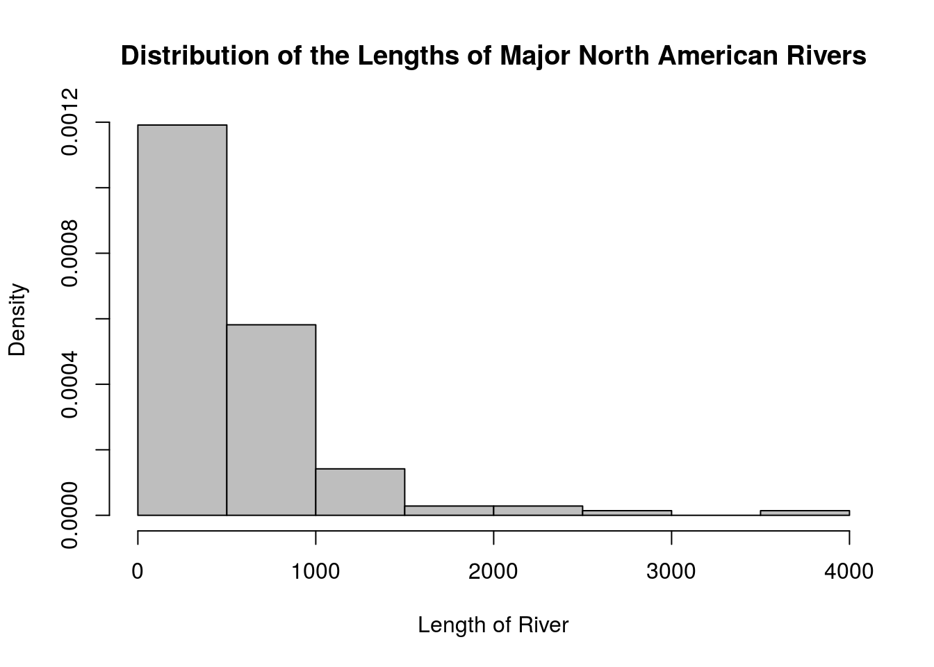
Density Curve
A density curve is another way to view a distribution where the end result is a smooth curve, It can be interpreted like a histogram, but it avoids disadvantages that come with choosing discrete classes. You can create a density curve with plot(density(x)).
plot(density(rivers), main = "Distribution of Lengths of Rivers")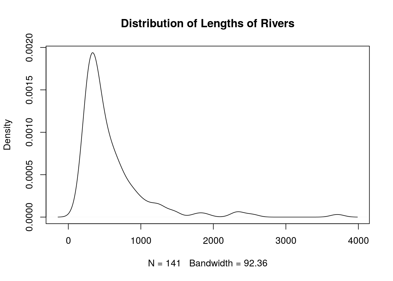
# It is possible to superimpose a density plot on top of a histogram to see the relationship. Just be sure that the histogram is showing relative frequencies rather than frequencies. Here is an example.
hist(rivers, main = "Distribution of the Lengths of Major North American Rivers",
     xlab = "Length of River",
     freq = FALSE,
     right = TRUE,
     breaks = round(sqrt(length(rivers))), # Using the sqrt(n) rule
     col = "gray",
     ylim = c(0, 0.0025)) # ylim sets the limits of the vertical axis
lines(density(rivers))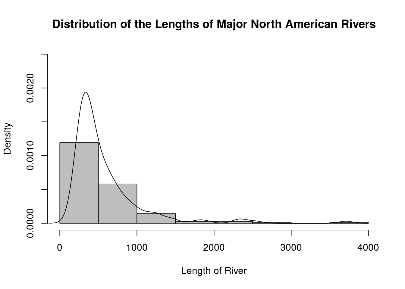
Boxplot
You can create a boxplot in R with the boxplot() function.
boxplot(rivers)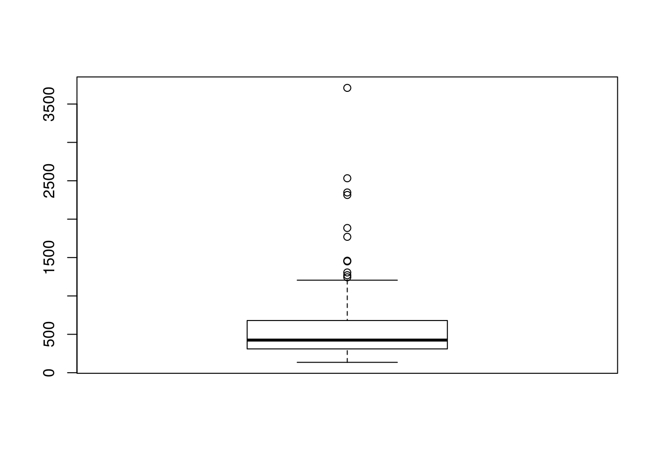
One of the major advantages of boxplots is being able to compare distributions of different samples. To do so, issue a call to boxplot() of the form boxplot(x ~ y), where x is a data vector with all samples combined, and y is a character or factor vector identifying the sample each element of x belongs to.
# I will be working with the iris dataset for this example
# Looking at the data
str(iris)
## 'data.frame': 150 obs. of 5 variables:
## $ Sepal.Length: num 5.1 4.9 4.7 4.6 5 5.4 4.6 5 4.4 4.9 ...
## $ Sepal.Width : num 3.5 3 3.2 3.1 3.6 3.9 3.4 3.4 2.9 3.1 ...
## $ Petal.Length: num 1.4 1.4 1.3 1.5 1.4 1.7 1.4 1.5 1.4 1.5 ...
## $ Petal.Width : num 0.2 0.2 0.2 0.2 0.2 0.4 0.3 0.2 0.2 0.1 ...
## $ Species : Factor w/ 3 levels "setosa","versicolor",..: 1 1 1 1 1 1 1 1 1 1 ...iris$Sepal.Length## [1] 5.1 4.9 4.7 4.6 5.0 5.4 4.6 5.0 4.4 4.9 5.4 4.8 4.8 4.3 5.8 5.7 5.4
## [18] 5.1 5.7 5.1 5.4 5.1 4.6 5.1 4.8 5.0 5.0 5.2 5.2 4.7 4.8 5.4 5.2 5.5
## [35] 4.9 5.0 5.5 4.9 4.4 5.1 5.0 4.5 4.4 5.0 5.1 4.8 5.1 4.6 5.3 5.0 7.0
## [52] 6.4 6.9 5.5 6.5 5.7 6.3 4.9 6.6 5.2 5.0 5.9 6.0 6.1 5.6 6.7 5.6 5.8
## [69] 6.2 5.6 5.9 6.1 6.3 6.1 6.4 6.6 6.8 6.7 6.0 5.7 5.5 5.5 5.8 6.0 5.4
## [86] 6.0 6.7 6.3 5.6 5.5 5.5 6.1 5.8 5.0 5.6 5.7 5.7 6.2 5.1 5.7 6.3 5.8
## [103] 7.1 6.3 6.5 7.6 4.9 7.3 6.7 7.2 6.5 6.4 6.8 5.7 5.8 6.4 6.5 7.7 7.7
## [120] 6.0 6.9 5.6 7.7 6.3 6.7 7.2 6.2 6.1 6.4 7.2 7.4 7.9 6.4 6.3 6.1 7.7
## [137] 6.3 6.4 6.0 6.9 6.7 6.9 5.8 6.8 6.7 6.7 6.3 6.5 6.2 5.9iris$Species## [1] setosa setosa setosa setosa setosa setosa
## [7] setosa setosa setosa setosa setosa setosa
## [13] setosa setosa setosa setosa setosa setosa
## [19] setosa setosa setosa setosa setosa setosa
## [25] setosa setosa setosa setosa setosa setosa
## [31] setosa setosa setosa setosa setosa setosa
## [37] setosa setosa setosa setosa setosa setosa
## [43] setosa setosa setosa setosa setosa setosa
## [49] setosa setosa versicolor versicolor versicolor versicolor
## [55] versicolor versicolor versicolor versicolor versicolor versicolor
## [61] versicolor versicolor versicolor versicolor versicolor versicolor
## [67] versicolor versicolor versicolor versicolor versicolor versicolor
## [73] versicolor versicolor versicolor versicolor versicolor versicolor
## [79] versicolor versicolor versicolor versicolor versicolor versicolor
## [85] versicolor versicolor versicolor versicolor versicolor versicolor
## [91] versicolor versicolor versicolor versicolor versicolor versicolor
## [97] versicolor versicolor versicolor versicolor virginica virginica
## [103] virginica virginica virginica virginica virginica virginica
## [109] virginica virginica virginica virginica virginica virginica
## [115] virginica virginica virginica virginica virginica virginica
## [121] virginica virginica virginica virginica virginica virginica
## [127] virginica virginica virginica virginica virginica virginica
## [133] virginica virginica virginica virginica virginica virginica
## [139] virginica virginica virginica virginica virginica virginica
## [145] virginica virginica virginica virginica virginica virginica
## Levels: setosa versicolor virginicaboxplot(iris$Sepal.Length ~ iris$Species)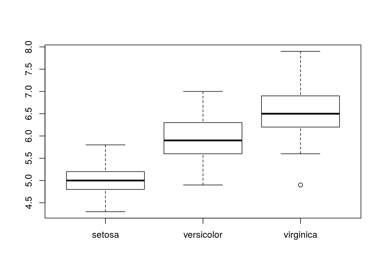
Bar Chart
For a categorical dataset, we can create a bar chart using the barchart() function. This is a natural way to visualize categorical data.
# Shows the cloudiness of different days in Central Park
barchart(central.park.cloud)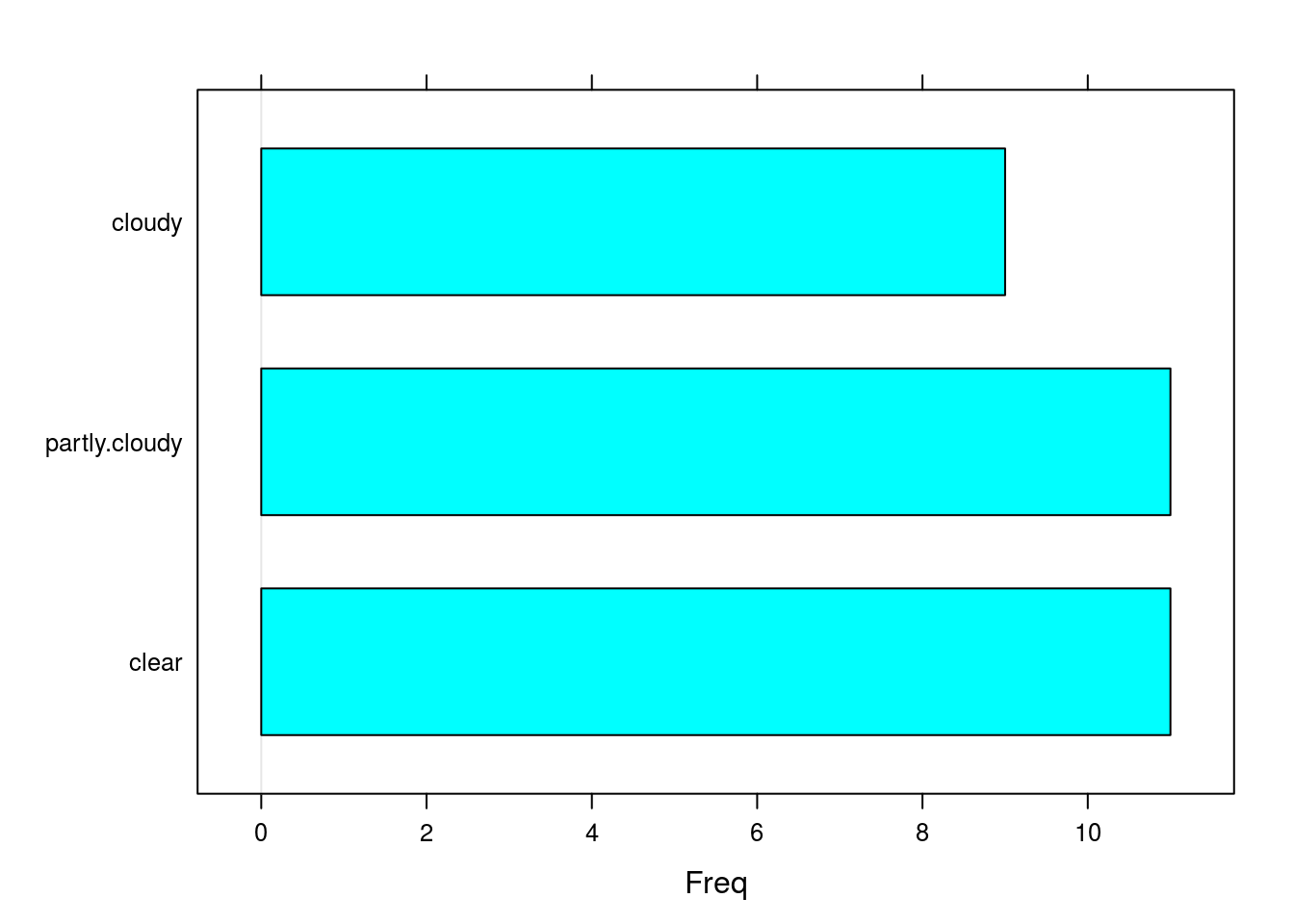
Numerical Summaries
A numerical summary tries to describe some aspect of a dataset using numbers. Two classes of numerical summaries include measures of location and measures of spread. There are many other numerical summaries (the textbook used in this lab describes measures of skewness and kurtosis in addition to measures of location and spread), but we will focus on these two.
First, a great way to obtain appropriate numerical summaries for a dataset is with the summary() function. This is a generic function that changes its behavior depending on the object passed to it. If x is a numeric vector, summary(x) will compute the five-number summary of x (minimum, first quartile, median, third quartile, maximum) in addition to the mean of x. On the other hand, if x is a factor or character vector, summary(x) will compute the frequency of each category in x. Thus, if you have a dataset you are unfamiliar with, summary() is a good way to see some basic information about it.
# Some basic information about rivers, a numeric dataset
summary(rivers)
## Min. 1st Qu. Median Mean 3rd Qu. Max.
## 135.0 310.0 425.0 591.2 680.0 3710.0# Frequencies for cloud conditions in central.park.cloud, a factor vector
summary(central.park.cloud)## clear partly.cloudy cloudy
## 11 11 9Of course it is possible to compute specific numeric summaries.
The mean of a dataset is defined as:
\[\bar{x} = \frac{\sum_{i=1}^{n} x_i}{n}\]
where \(x_i\) is the \(i^{\text{th}}\) observation and \(n\) the size of the dataset. The mean can be computed in R using the mean() function. To obtain the trimmed mean, you can set the trim parameter to a value between 0 and 0.5; this sets how much of the data to “trim” from either end of the ordered dataset. If trim = 0 (the default), no data is trimmed from either end, but if trim = 0.5, as much data is possible is trimmed from either end and the median is computed.
# The mean executive pay (in $10,000's)
mean(exec.pay)## [1] 59.88945# There are very large outliers, though; what happens to the mean if we trim
# 10% of the data from either side of the (ordered) dataset?
mean(exec.pay, trim = 0.1)## [1] 29.96894The median is the number that splits the dataset in half after being ordered. You can compute the median in R using the median() function.
# The median executive pay; compare to the mean or trimmed mean
median(exec.pay)## [1] 27The \((100\alpha)^{\text{th}}\) percentile is the number such that \(100\alpha\%\) of the dataset lies below and \(100(1-\alpha)\%\) above the number. The quantile() function in R computes percentiles (also referred to as quantiles). quantile(x) will effectively find the five-number summary of the dataset x, including the first and third quartiles. Alternatively, one can call quantile(x, p), where p is a vector (or perhaps just a number that will be interpreted as a vector) specifying with percentiles are wanted (these are numbers between 0 and 1).
The fivenum() function will find five-number summaries outright, but one may as well call quantile() with the default parameters (the presentation is better anyway).
# The five-number summary using fivenum
fivenum(exec.pay)## [1] 0.0 14.0 27.0 41.5 2510.0# The same information using quantile
quantile(exec.pay)## 0% 25% 50% 75% 100%
## 0.0 14.0 27.0 41.5 2510.0# What is the 99th percentile of executive pay?
quantile(exec.pay, .99)## 99%
## 906.62# The deciles of exec.pay, breaking the dataset into 10 parts
quantile(exec.pay, seq(0, 1, by = .1))## 0% 10% 20% 30% 40% 50% 60% 70% 80% 90%
## 0.0 9.0 12.6 16.0 22.0 27.0 31.0 38.0 48.0 91.4
## 100%
## 2510.0Now let’s discuss measures of spread. The range of a dataset is the difference between the largest and smallest values:
\[\text{range} = \max_i x_i - \min_i x_i\]
R’s range() function will find the maximum and minimum of the dataset, but won’t difference them. This is not a problem, though; simply call diff() on the result of range to subtract the minimum from the maximum, like diff(range(x)), where x is the dataset.
# The largest and smallest executive pay
range(exec.pay)## [1] 0 2510# The range
diff(range(exec.pay))## [1] 2510Another (more common) means for numerically describing the spread of a dataset is with the standard deviation or its square, the variance. The variance is defined as follows:
\[s^2 = \frac{1}{n - 1}\sum_{i = 1}^{n}(x_i - \bar{x})^2\]
The standard deviation is merely the square root of the variance.
\[s = \sqrt{s^2}\]
In R, the function var() finds a dataset’s variance, and sd() finds the standard deviation.
# The variance of exec.pay
var(exec.pay)## [1] 42867.03# We could take the square root of the variance to get the standard
# deviation
sqrt(var(exec.pay))## [1] 207.0435# Or we could just use sd
sd(exec.pay)## [1] 207.0435For categorical data, the simplest way to numerically summarize the data is with a table. We can create one with the table() function
table(central.park.cloud)## central.park.cloud
##         clear partly.cloudy        cloudy
## 11 11 9# Create a frequency table by dividing a table by the sample size (i.e. the
# length of the data vector)
table(central.park.cloud)/length(central.park.cloud)## central.park.cloud
## clear partly.cloudy cloudy
## 0.3548387 0.3548387 0.2903226
Comments
You may have noticed already the
#symbol in the code. This is called a comment. The R interpreter completely ignores comments. They are used for annotating code. Commenting is not optional; it’s essential to understanding code when it is read (and I promise you, it will be). You can’t write good code without comments. Consequently, I require you to write good, extensive comments in your homework!