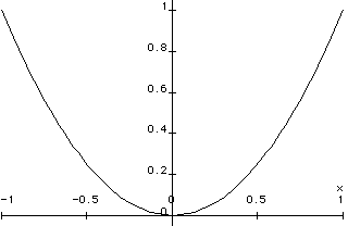
plot( x^2, x = -1..1 );
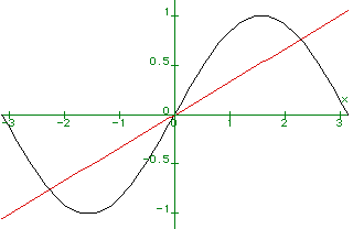
plot( { sin(x), (1/3)*x }, x = -Pi..Pi );
By looking at the graph we can solve the equation sin(x) = x/3. The roots are determined by the places where the two curves cross.
We can graph surfaces using the plot3d command. For example, to graph z = xy, where x and y run from -1 to 1, we do this:
plot3d( x*y, x=-1..1, y=-1..1, axes = BOXED, style = PATCH);
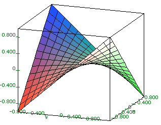
For more information use the ?plot3d command. No semicolon needed for this one.
   solve(x^3 = 27);

                                    1/2                 1/2
                  3, - 3/2 + 3/2 I 3   , - 3/2 - 3/2 I 3
Note that there are three solutions, two of which are complex. Now let's try something more complicated:
    solve(x^3 + 1.5*x = 27);

                2.83,  - 1.42 + 2.74 I,  - 1.42 - 2.74 I
Note: There is a good reason why we wrote "1.5 " instead of "(3/2)" as the coefficient of x in the last equation. If one of the numbers in the equation is in decimal form, then Maple tries to find an approximate solution in decimal form. If none of the numbers are in decimal form, as in the first example, then Maple tries to find an exact solution. This may fail, since there is no algebraic formula for the roots polynomial equations of degree five or more ( Galois ).
   solve( { 2*x + 3*y = 1, 3*x + 5*y = 1} );

                               {y = -1, x = 2}
These can contain literal as well as numerical coefficients:
   solve( { a*x + 5*y = 1, 3*x + b*y = c}, { x, y } );

                           - 3 + a c         - b + 5 c
                     {y = ----------, x = - ----------}
                          - 15 + a b        - 15 + a b
In the second example we have to tell Maple that x and y are the variables to be solved for. Otherwise it wouldn't know.
You can solve systems of two equations in two unknowns of the form f(x) = 0, g(x) = 0 by graphing the functions f(x) and g(x) and seeing where the curves cross.
Maple does arithmetic pretty much as you would expect it to:
3*(1.3 + 1.7)^2/2 - 0.1;
                                 13.400000000
It has built-in commands which can do a lot of work quickly. For example, to add up the numbers 1, 1/2, 1/3, ... 1/10, we do this:
   > sum(1/n, n= 1..10);
                                    7381
                                    ----
                                    2520
Note that Maple gave us the exact answer as a fraction in lowest terms. For an approximate answer in decimal form, do this:
   > sum(1.0/n, n= 1..10);
                                    2.928968254
The only difference was the 1.0 in place of 1 . Note the decimal point. We can also things like factor numbers:
   > ifactor(123456789);
                                2
                             (3)  (3803) (3607)
   > p := (a+b)^2;  # define p to be the square of (a + b)

                                             2
                                 p := (a + b)

   > expand(p);     # expand it

                                 2            2
                                a  + 2 a b + b


   > factor(a^2 + 2*a*b + b^2);

                                           2
                                    (a + b)

   > a := 1;  # define a to be 1

                                     a := 1

   > p;  # re-evaluate p

                                           2
                                    (1 + b)

   > a := 'a';  # define a to be a again

                                     a := a

   > p;  # check it out

                                           2
                                    (a + b)
   > sin(Pi/2);

                                       1

   > arcsin(1);

                                     1/2 Pi
We can set things up for conversions like this:
   > deg := evalf(Pi/180);  # use evalf to convert to decimal form

                              deg := .01745329252

   > rad := 1/deg;

                               rad := 57.29577951

   > sin(90*deg);

                                       1.

   > arcsin(1)*rad;

                                 28.64788976 Pi

   > evalf(");  # " stands for the result of the preceding computation

                                  90.00000002
Note two things. Sometimes we need to use the evalf function to convert results from exact to floating point (decimal) form. Sometimes it is convenient to use the quote(") sign: it stands for the result of the preceding computation.
   > f := x -> sqrt( 1 + x^2 );

                                                 2
                             f := x -> sqrt(1 + x )

   > f(1);

                                       1/2
                                      2
   > f(a+3);

                                      2       1/2
                               (10 + a  + 6 a)
These can have more than one variable:
   > g := (x,y) -> sqrt(x^2 + y^2);

                                              2    2
                          g := (x,y) -> sqrt(x  + y )

   > g(3,4);

                                       5
   > diff( sin(cos(x)) + x^3 + 1, x );
                                                   2
                         - cos(cos(x)) sin(x) + 3 x
It can do both definite and indefinite integrals:
   > int( x^2, x );
                                        3
                                   1/3 x
   > int( x^2, x = 0..1);
                                     1/3

   > evalf( int( sqrt( 1 + x^3 ), x = 0..1 ) );
                                 1.111447971
The last computation deserves comment. Suppose we just do the obvious thing (try it!).
> int( sqrt( 1 + x^3 ), x = 0..1 ):
Maple does not give us a numerical answer because the integral of this function cannot be expressed in terms of elementary functions. In particular it cannot be integrated by the usual techniques. However, note that we have surrounded our computation with evalf( ... ). This forces Maple to evaluate the integral numerically: evalf stands for evaluate in floating point form
Here are some examples of matrix calculations. Be sure to use with(linalg) before doing them. Also be sure to try these out to see how they work!
   > with(linalg):
   > a := matrix([
               [1, 2],
               [3, 4]
            ]);
   matrix is displayed ........
   > b := matrix([
               [0, 1],
               [1, 0]
            ]);
   ........
   > multiply( a, b );
   ........
   > multiply( b, a );
   ........
   > evalm( b &* a );  # another way of computing ba
   ..........
   > ?evalm # consult help on evalm
   > aa := inverse( a );
    ........
   > c := randmatrix(2,2); # 2x2 random matrix
   > evalm( 1/c ); # invert it
   > print( aa );  # redisplay aa
   ........
Did you notice the difference between the product ab and the product ba?
For information and examples on a particular Maple " function", use the "?" command. For example,
> ?solve
gives information on the solve command. Often it is helpful to scroll to the end of the help window and look at the examples, bypassing the technical discussion that precedes it. You can also try the command with no keyword:
> ?
This gives additonal information on how to use the help system.
Back to Maple
Back to Department of Mathematics, University of Utah
Last modified by
jac
March 27, 1995
Copyright © 1995 Department of Mathematics, University
of Utah