next state = f( current state )
The funcion f determines the behavior of the system. From it we
can calculate future states from prior ones.
Example Let f(x) = 2x define the chage-of-state function, and let x_0 = 1 be the population at time t = 0. (The unit of time is, say, one hour, and the unit of population is, say, one thousand (bacteria)). The we compute future states as follows:
  x_1 = f(x_0) = 2 x 1 = 2
  x_2 = f(x_1) = 2 x 2 = 4
  x_3 = f(x_2) = 2 x 4 = 8
  x_4 = f(x_3) = 2 x 8 = 16
In this case it is quite easy to guess what the general pattern is:
x_n = f^n(x_0) = 2^nHere "f^n(x)" means "the result of applying f to x a total of n times". Thus f^3(x) = f(f(f(x))).
The model of population growth just discussed is one in which the growth is exponential: we can write
x_n = exp( n log(2) )where "log" is the natural logarithm. This is not a realistic model over long periods of time since the population quickly grows to absurd sizes.
Problem: A typical spherical bacterium is about one micron (one millionth of a meter) in diameter. Assuming a one-hour doubling time, compute the time needed for a single bodacious bacterium to (a) completely cover the surface of the earth, (b) completely fill the volume of the earth.
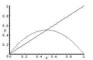
A somewhat more realistic model of population growth is given by a function f whose graph is convex downard, as in the figure below:

This is the graph of the function f(x) = 2x(1 - x). We notice that for very small values of x, corresponding to small populations, the graph of f is close to the tangent line at the origin, given by y = 2x. Thus, for small populations, we expect our new model to behave like the old one. However, note (from the graph), that if x > 1/2, then f(x) < x. Thus, if the population exceeds a certain critical value p = 1/2 units, then the next value of the population is smaller: the population declines. This is quite unlike the behavior of the first model.
The critical value p is a fixed point: it is a solution of the equation
f(p) = pA fixed point has the property that if the state at a certain time is p, then it will be p for all future time. It is therefore a "rest", or equilibrium state.
Problem. Suppose that f(x) = 3x(1-x). What are the fixed points?
When the change-of-state function is quadratic, as opposed to linear, simple formulas for x_n in terms of x_0 are not known. Nevertheless, it is possible to understand many things about the sequence { x_n }. We will use both analytic and computional tools in the problems below.
Your program should produce screen output something like this:
  x_0 = 0.100

  0.189  0.322  0.458  0.521  0.524  0.524  0.524  0.524  0.524  0.524
  0.524  0.524  0.524  0.524  0.524  0.524  0.524  0.524  0.524  0.524
You may wish to start with the following outline for the program. Remember: start simple, get the basics working, then refine the program.
/***************************************************************
  Define the constant k and the function f:
***************************************************************/

double k;

double f( double x ) {
  return k*(1-x)*x;
}

main()
{

/***************************************************************
  Declare x, the current state, n, the number of iterations,
  and i, the loop counter.
***************************************************************/

double x, n;
int i;


/*  Initialize variables, print x */

/*  Loop to update and print x */


}
  0 x_0
  1 x_1
  2 x_2
  etc.
To plot the data in the file we may use Maple's readdata and plot commands .
Continue the analysis of previous problem after making graphs for each of the sequence { x_n }.
In class we studied the sequences { x_n } produced by the dynamical system with generating function f(x) = kx(1-x) for various choices of the initial state x_0 and of the constant k. We found that as k changes, the behavior of the sequence changes. For example: