• Your final exam, project and final grade for the class have been sent to you via email. Graded papers may be picked up during my office hours in the Spring (MTW 2-3pm) or in Math 5620.
• Some histograms
  Letter grade Final exam grade A :***** 110:*** A-:***** 100:****** B+:*** 90:*** B :**** 80: B-:*** 70:*** C+:* 60:* C :* 50:* 40:** 30:**

• The practice final solution is here: final_practice_sol.pdf
• The solutions to HW7 are here: hw07_sol.pdf

• Here is a practice final: practice_final.pdf. It is longer and more difficult than the actual final and contains typical problems. We will solve this together on the Wed and Thu lectures.

• HW6 solutions are here: hw06_sol.pdf.
• A review sheet for the final is here: final_study_sheet.pdf. Please look at it and bring questions or areas you want to review for the Mon and Tue lectures.
• The Wed and Thu lectures will be devoted to solving a practice final (which will be posted soon).
• As a friendly reminder:
  • The final is on Wed Dec 14 10:30am-12:30pm in our usual classroom (JTB 130).
  • The exam starts at 10:30am sharp. No extra time will be given if you come late, so plan to come at least 5 minutes early.
  • The exam is closed book and no calculators are allowed (or needed). No notes are allowed except for the equivalent of two letter sized, single sided, handwritten cheat sheets.

• Homework 7 is due on Tue Dec 6 and is here: hw07.pdf. The accompanying stubs are: mylu.m and test_mylu.m.

• Here are the FFT demos we did in class: sounddemo.m (shows how to filter a sound signal using the FFT) and imdemo.m (gives the rough idea behind lossy compression as used in e.g. JPEG). These demos will not run unmodified in Octave. You need at least to provide your own sound or image samples to work with.
• This week we started looking at direct methods for solving linear systems (Chap 6). The notes for this week and next week are here: math5610_013.pdf and math5610_014.pdf.
• Here is tentatively what to expect for the last two weeks of classes:
  • Finish chapter 6 (LU, Cholesky, sparse systems)
  • HW7 will be posted on Mon 11/28 and due in a week. It will cover Chap 6.
  • A practice final and review sheet will be posted in the next week of classes
  • In the last week of classes expect:
    • 1-2 lectures for solving practice final exam
    • 1-2 review lectures

• Here are the class notes for the Fast Fourier Transform: math5610_012.pdf.
• Here is a recursive (and not very efficient) implementation of the FFT: myfft.m and a test against Matlab’s FFT: test_myfft.m.

• HW6 is due on Wed Nov 23 and is available here: hw06.pdf. The sample code is here: prob1_sample.m

• Here are the class notes for last week and also for this week: math5610_009.pdf (Romberg integration, adaptive Simpson integration), math5610_010.pdf (linear algebra preliminaries) and math5610_011.pdf (Chapter 8: Approximation theory. Includes discrete least squares, best approximation theory, Chebyshev polynomials, Fourier series)
• Note: The page numbers in red take precedence over the handwritten ones.

• The second part of this class is Math 5620 which is offered in the Spring 2012 MTWF 10:45-11:35am (see the Math course schedules). The instructor will be myself and we will use the same textbook as in Math 5610.
  • The program until the end of the year for Math 5610 is: Ch 6-7 (solving linear systems), Ch 8 (Approximation theory, least squares).
  • The program for Math 5620 is roughly: Ch 9 (eigenvalue algorithms), Ch 5 (ODEs, initial value problems), Ch 11 (Boundary value problems), Ch 12 (Finite differences and Finite elements)
• Reminder: You need to send me your choice of group and project by Nov 7. If you have not found a group there are two options:
  • If you are comfortable working by yourself in one of the projects and you are confident you can finish it, you can do the project by yourself. You need to tell me about this.
  • If you prefer working in a group, email me your project preference and I will assign you to work with someone else that does not have a group.

• HW5 is here hw05.pdf and is due Tue Nov 8. Sample code for Problem 1 is here: prob1.m.
• The plot for Problem 1 should be similar to this one:
  

• The suggested projects are here: projects.pdf.
• You need to choose a group of 2-3 persons and tell me your choice by Nov 7.
• One project report per group is due Thu Dec 9.

• Class notes for last week are here: math5610_007.pdf (Hermite interpolation, cubic splines) and math5610_008.pdf (Numerical differentiation and integration. Newton-Cotes quadratures, composite quadratures, Guassian quadrature).
• The next HW will be posted next Monday.

• The solutions to yesterday’s midterm are here: midterm_sol.pdf.
• The histogram of the grades of this homework (which is graded over 90) is:
  

   30: *
   40: **
   50: *
   60: **
   70: *********
   80: ********
   90: *
  100:
  110: *
  

  * You should have received an email with your HW and Midterm grades. It includes a Partial Grade which is computed by weighting 65% the HW average and 55% the midterm. This should have been 55% and 45%. The histogram for the updated partial grades (over 100) is below. Another email with the correct ratios will be sent.
  

   50: **
   60: ****
   70: ******
   80: ****
   90: *******
  100: 
  110: *
  

• Due to a gas leak in JTB, today’s midterm is rescheduled for tomorrow Wed 10/19.

• HW4 solutions are here: hw04_sol.pdf.
• As a reminder: the midterm exam is tomorrow in class. Please plan on coming 5min earlier.

• Practice Midterm Solutions are here: midterm_practice_sol.pdf.

• HW3 solutions are here: hw03_sol.pdf.

• Here is a practice midterm: midterm_practice.pdf and the study sheet for the midterm: study_sheet.pdf. Please keep in mind the Practice Midterm is about 1.5 times longer and a more difficult than the actual midterm.
• HW4 may be turned in until Fri Oct 14.

• Solutions to HW2 are here: hw02_sol.pdf
• In HW 4 Problem 1: Do not use Matlab’s sign to write the quadratic formula (as is done in the equation immediately above Algorithm 2.8 in your book, which I call from now on Eq. (A)). The problem with sign is that it has a meaning for complex numbers. What you can do is evaluate the denominator of Eq. (A) with both a plus and a minus sign and determine which sign gives the largest one (Step 4 in Algorithm 2.8). The new guess of the root will be the solution with the largest denominator of Eq. (A) (Step 5 in Algorithm 2.8).
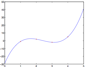
• For HW4 Problem 3: The output of newtondd.m is assumed to be a vector with the coefficients of the Newton interpolation polynomial. To test your code you may use the code from help newtondd, which is:

  x  = linspace(0,5);
  xd = [1 2 3 4];
  yd = [-1 2 -2 5];
 
  d = newtondd(xd,yd);
  y = newtonev(xd,d,x);
  plot(x,y,xd,yd,'r+')

The plot you should get looks like this one:

• HW4 is due Wed Oct 5 and is available here: hw04.pdf. Sample codes and sutubs are here:
  • prob1.m – driver for problem 1 (Müller’s method)
  • muller.m – actual implementation of Müller’s method.
  • horner.m – Horner’s method for evaluating a polynomial (from last homework). This is used in Müller’s method.
  • prob3.m – driver for problem 3 (polynomial interpolation)
  • newtondd.m – computes coefficients in Newton form of interpolation polynomial using divided differences
  • newtonev.m – evaluates interpolation polynomial in Newton form
  • lagrange.m – evaluates interpolation polynomial in Lagrange form
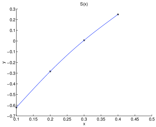
  • In the sample problem 3, the plot you get should be similar to
    
• Class notes for the past week are here: math5610_005.pdf and math5610_006.pdf.

• HW3 is now due on Thu Sep 29 because of problems running Matlab in the Math department system.
• HW4 will still be posted on Tuesday.

• The midterm exam will be this Tue Oct 18 in class. Here is what to expect:
  • Mon Oct 3: Practice exam and study sheet posted.
  • Thu Oct 6 and Mon Oct 17: Solution of practice exam and Q&A session.
  • The exam is closed book and no calculators are allowed (or needed). No notes are allowed except for a letter sized, single sided, handwritten cheat sheet.
• For HW3 Problem 1:
  • For the stopping criterion, please do not use function values, i.e. abs(f(x)) <= TOL, as your code may terminate early (in the sample problem the initial guess does actually satisfy this stopping criterion). Please use the stopping criterion abs(x-xnew) <= TOL.
  • The B&F book has a typo in 2.4.2 b. The function to consider should be x^6 + 6*x^5 + 9*x^4 + ... (the first term is x^2 in the book, which does not give a multiple root)

• The updated HW3 is available here: hw03.pdf. The only changes are:
  • Problem 1: Only need to do cases a and b
  • Problem 5: Corrected references to Theorems in ninth edition. Part a is very similar to HW2 Problem 6. Part b is simpler in the polynomial case.
  • Fixed typo in the sample output of prob2.m

• HW3 is due Tue Sep 27 and is available here: hw03.pdf. Sample code and stubs are here:
  • fixedpoint.m – stub for Fixed point iteration
  • steffensen.m – stub Steffensen’s acceleration
  • prob1.m – sample driver for problem 1
  • newton.m – stub for Newton’s method (you may use the code your wrote for HW2)
  • newton_mult.m – stub for Modified Newton’s method for multiple roots.
  • prob2.m – sample driver for problem 2
  • horner.m – stub for Horner’s method
  • hornernm.m – stub for specialized Horner’s method (to be used in polynm.m)
  • polynm.m – stub for Newton’s method specialized to polynomials (uses hornernm to compute efficiently value of polynomial and derivative at the current iterate)
  • prob3.m – sample driver for problem 3
• Solutions to HW1 are here: hw1_sol.pdf.

• HW2 is here: hw02.pdf and is due Tue Sep 20.
• The sample Matlab drivers for HW2 are here: prob1_sample.m, prob3_sample.m. Some stubs for the different methods you need to implement are here: bisect.m, newton.m, secant.m.
• The code for last weeks computer lab is here: cl02_p1.m.
• The class notes for last week and this week are here: math5610_003.pdf, math5610_004.pdf. Today we covered Aitken’s acceleration and Steffensen’s method and we just barely started talking about polynomials.
• As a reminder: We meet tomorrow Wed Sep 14 in the Computer Lab LCB 115.

• Homework 1 is due on Tue Sep 13 in class and is available here: hw01.pdf.
• We have a computer lab at the usual time in LCB 115 on:
  • Wed Sep 7
  • Wed Sep 14
• Class notes for last week are here: math5610_002.pdf.
• The code for computer lab 1 is here: logtaylor1.m, logtaylor2.m, computerlab1.m. The latter file is slightly more complicated (but more general) than what we actually did in the computer lab.

• Here are the instructions for the last Computer Lab: computerlab01.pdf and for today’s computer lab: computerlab02.pdf.
• Here is the file we created last time in Matlab: logtaylor1.m
• Here are some Matlab tutorials:
  • A Matlab primer by Kermit Sigmon
  • Matlab tutorial from Scientific Computing and Visualization, Boston University
  • Matlab tutorial from Math department, University of Utah
• Here are some instructions on how to obtain and/or install Matlab or Octave.

• The class notes for last week are here: math5610_001.pdf. We covered some preliminaries (limits, continuity, Mean Value Theorem, Taylor’s theorem, big O and little o notation) and floating point arithmetic.
• The next computer lab will be on Wed Aug 31 in LCB 155 at the usual class time.
• There is no homework assigned this week.

• You should shortly receive an email through your University of Utah account (a.k.a. Umail). If you prefer to get the class announcements in another email address, please consider forwarding your Umail using the uNID account tools at https://unid.utah.edu/.
• The following lectures will be held at the Computer Lab in LCB 115
  • Thursday Aug 25
  • Tuesday Aug 30 Wednesday Aug 31 (UPDATED)

Announcements, assignments and other class information will be posted here.